8.4 – What Causes Changes in Unemployment over the Short Run

We have seen that unemployment varies across times and places. What causes changes in unemployment? There are different answers in the short run and in the long run. Let’s look at the short run first.

Cyclical Unemployment

Let’s make the plausible assumption that in the short run, from a few months to a few years, the quantity of hours that the average person is willing to work for a given wage does not change much, so the labour supply curve does not shift much. In addition, make the standard ceteris paribus assumption that there is no substantial short-term change in the age structure of the labour force, institutions and laws affecting the labour market, or other possibly relevant factors.

One primary determinant of the demand for labour from firms is how they perceive the state of the macro economy. If firms believe that business is expanding, then at any given wage they will desire to hire a greater quantity of labour, and the labour demand curve shifts to the right. Conversely, if firms perceive that the economy is slowing down or entering a recession, then they will wish to hire a lower quantity of labour at any given wage, and the labour demand curve will shift to the left. Economists call the variation in unemployment that the economy causes moving from expansion to recession or from recession to expansion (i.e. the business cycle) cyclical unemployment.

From the standpoint of the supply-and-demand model of competitive and flexible labour markets, unemployment represents something of a puzzle. In a supply-and-demand model of a labour market, as Figure 8.4a illustrates, the labour market should move toward an equilibrium wage and quantity. At the equilibrium wage (We), the equilibrium quantity (Qe) of labour supplied by workers should be equal to the quantity of labour demanded by employers.

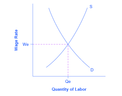
The graph reveals the complexity of unemployment in that, presumably, the number of jobs available should equal the number of individuals pursuing employment. Probably a few people are unemployed because of unrealistic expectations about wages, but they do not represent the majority of the unemployed. Instead, unemployed people often have friends or acquaintances of similar skill levels who are employed, and the unemployed would be willing to work at the jobs and wages similar to what those people are receiving. However, the employers of their friends and acquaintances do not seem to be hiring. In other words, these people are involuntarily unemployed. What causes involuntary unemployment?

Why Wages Might Be Sticky Downward

If a labour market model with flexible wages does not describe unemployment very well—because it predicts that anyone willing to work at the going wage can always find a job—then it may prove useful to consider economic models in which wages are not flexible or adjust only very slowly. In particular, even though wage increases may occur with relative ease, wage decreases are few and far between.

One set of reasons why wages may be “sticky downward,” as economists put it, involves economic laws and institutions. For low-skilled workers receiving minimum wage, it is illegal to reduce their wages. For union workers operating under a multiyear contract with a company, wage cuts might violate the contract and create a labour dispute or a strike. However, minimum wages and union contracts are not a sufficient reason why wages would be sticky downward for the U.S. economy as a whole. After all, out of the 150 million or so employed workers in the U.S. economy, only about 2.6 million—less than 2% of the total—do not receive compensation above the minimum wage. Similarly, labour unions represent only about 11% of American wage and salary workers. In other high-income countries, more workers may have their wages determined by unions or the minimum wage may be set at a level that applies to a larger share of workers. However, for the United States, these two factors combined affect only about 15% or less of the labour force.

Economists looking for reasons why wages might be sticky downwards have focused on factors that may characterize most labour relationships in the economy, not just a few. Many have proposed a number of different theories, but they share a common tone.

One argument is that even employees who are not union members often work under an implicit contract, which is that the employer will try to keep wages from falling when the economy is weak or the business is having trouble, and the employee will not expect huge salary increases when the economy or the business is strong. This wage-setting behavior acts like a form of insurance: the employee has some protection against wage declines in bad times, but pays for that protection with lower wages in good times. Clearly, this sort of implicit contract means that firms will be hesitant to cut wages, lest workers feel betrayed and work less hard or even leave the firm.

Efficiency wage theory argues that workers’ productivity depends on their pay, and so employers will often find it worthwhile to pay their employees somewhat more than market conditions might dictate. One reason is that employees who receive better pay than others will be more productive because they recognize that if they were to lose their current jobs, they would suffer a decline in salary. As a result, they are motivated to work harder and to stay with the current employer. In addition, employers know that it is costly and time-consuming to hire and train new employees, so they would prefer to pay workers a little extra now rather than to lose them and have to hire and train new workers. Thus, by avoiding wage cuts, the employer minimizes costs of training and hiring new workers, and reaps the benefits of well-motivated employees.

The adverse selection of wage cuts argument points out that if an employer reacts to poor business conditions by reducing wages for all workers, then the best workers, those with the best employment alternatives at other firms, are the most likely to leave. The least attractive workers, with fewer employment alternatives, are more likely to stay. Consequently, firms are more likely to choose which workers should depart, through layoffs and firings, rather than trimming wages across the board. Sometimes companies that are experiencing difficult times can persuade workers to take a pay cut for the short term, and still retain most of the firm’s workers. However, it is far more typical for companies to lay off some workers, rather than to cut wages for everyone.

The insider-outsider model of the labour force, in simple terms, argues that those already working for firms are “insiders,” while new employees, at least for a time, are “outsiders.” A firm depends on its insiders to keep the organization running smoothly, to be familiar with routine procedures, and to train new employees. However, cutting wages will alienate the insiders and damage the firm’s productivity and prospects.

Finally, the relative wage coordination argument points out that even if most workers were hypothetically willing to see a decline in their own wages in bad economic times as long as everyone else also experiences such a decline, there is no obvious way for a decentralized economy to implement such a plan. Instead, workers confronted with the possibility of a wage cut will worry that other workers will not have such a wage cut, and so a wage cut means being worse off both in absolute terms and relative to others. As a result, workers fight hard against wage cuts.

These theories of why wages tend not to move downward differ in their logic and their implications, and figuring out the strengths and weaknesses of each theory is an ongoing subject of research and controversy among economists. All tend to imply that wages will decline only very slowly, if at all, even when the economy or a business is having tough times. When wages are inflexible and unlikely to fall, then either short-run or long-run unemployment can result. Figure 8.4b illustrates this.

 

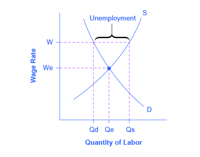
Figure 8.4b Sticky Wages in the Labour Market (Text Version)

The graph provides a visual of how sticky wages impact the unemployment rate. The vertical axis is Wage Rate and the horizontal axis is Quantity of Labour. The supply curve (S) slopes upward from left to right and the demand curve (D) slope downward from left to right. The equilibrium occurs where S and D intersect, at point We and Qe. The wage rate, point W, is stuck above the equilibrium;  as a result the number of those who want jobs (Qs) is greater than the number of job openings (Qd). Qs is greater then Qe and Qd is lesser then Qe.  Unemployment, shown by the bracket in the figure, spans between Qd and Qs at W.

Figure 8.4c shows the interaction between shifts in labour demand and wages that are sticky downward. Figure 8.4c (a) illustrates the situation in which the demand for labour shifts to the right from D₀ to D₁. In this case, the equilibrium wage rises from W₀ to W₁ and the equilibrium quantity of labour hired increases from Q₀ to Q₁. It does not hurt employee morale at all for wages to rise.

Figure 8.4c (b) shows the situation in which the demand for labour shifts to the left, from D₀ to D₁, as it would tend to do in a recession. Because wages are sticky downward, they do not adjust toward what would have been the new equilibrium wage (W₁), at least not in the short run. Instead, after the shift in the labour demand curve, the same quantity of workers is willing to work at that wage as before; however, the quantity of workers demanded at that wage has declined from the original equilibrium (Q₀) to Q₂. The gap between the original equilibrium quantity (Q₀) and the new quantity demanded of labour (Q₂) represents workers who would be willing to work at the going wage but cannot find jobs. The gap represents the economic meaning of unemployment.

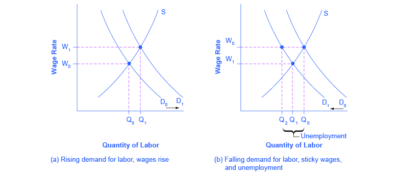
Figure 8.4c Rising Wage and Low Unemployment: Where Is the Unemployment in Supply and Demand? (Text Version)

There are two graphs that show how supply and demand influence unemployment. Both graphs have a vertical axis is Wage Rate and the horizontal axis is Quantity of Labour.

Graph A – Rising demand for labour, wages rise: In a labour market where wages are able to rise the supply curve (S) slopes upward from left to right and the original demand curve (D) slopes downward from left to right. The equilibrium occurs where the S and D intersect, at point W₀ and Q₀. An increase in the demand for labour shifts the original demand curve (D₀) to the right to D₁, resulting in equilibrium quantity of labour hired shifting to the right from Q₀ to Q₁ and a rise in the equilibrium wage from W₀ to W₁. The new equilibrium occurs where S and D₁ intersect at W₁ and Q₁ .

Graph B – Falling demand for labour, sticky wages, and unemployment: In a labour market where wages do not decline, a fall in the demand for labour occurs. The supply curve (S) slopes upward from left to right and the original demand curve (D) slopes downward from left to right. The equilibrium occurs where the S and D intersect, at point W₀ and Q₀. The original demand curve (D₀) shifts to the left to D1 resulting in a decline in the quantity of labour demanded at the original wage (W₀) shift to the left from Q₀ to Q₂. These workers will want to work at the prevailing wage (W₀), but will not be able to find jobs. The new equilibrium occurs where S and D₁ intersect at W₁ and Q₁. Q₁ occurs between Q₂ and Q₀. The span between Q₂ and Q₀ is unemployment.

This analysis helps to explain the connection that we noted earlier: that unemployment tends to rise in recessions and to decline during expansions. The overall state of the economy shifts the labour demand curve and, combined with wages that are sticky downwards, unemployment changes. The rise in unemployment that occurs because of a recession is cyclical unemployment.

Link It Up

The St. Louis Federal Reserve Bank is the best resource for macroeconomic time series data, known as the Federal Reserve Economic Data (FRED). FRED [New Tab] provides complete data sets on various measures of the unemployment rate as well as the monthly Bureau of Labor Statistics report on the results of the household and employment surveys.

Key Concepts and Summary

Cyclical unemployment rises and falls with the business cycle. In a labour market with flexible wages, wages will adjust in such a market so that quantity demanded of labour always equals the quantity supplied of labour at the equilibrium wage. Economists have proposed many theories for why wages might not be flexible, but instead may adjust only in a “sticky” way, especially when it comes to downward adjustments: implicit contracts, efficiency wage theory, adverse selection of wage cuts, insider-outsider model, and relative wage coordination.

Attribution

Except where otherwise noted, this chapter is adapted from “What Causes Changes in Unemployment over the Short Run” and “Key Concepts and Summary” In Principles of Economics 2e. (OpenStax) by Steven A. Greenlaw, David Shapiro, licensed under CC BY 4.0./Adaptations include addition of chapter key concepts and summary.

Access for free at Principles of Microeconomics 2e

Original Source Chapter References