4.4 – Labour and Financial Markets

The theories of supply and demand do not apply just to markets for goods. They apply to any market, even markets for labor and financial services. Labour markets are markets for employees or jobs. Financial markets are markets for saving or borrowing.

When we think about demand and supply curves in goods and services markets, it is easy to picture who the demanders and suppliers are: businesses produce the products and households buy them. Who are the demanders and suppliers in labor and financial service markets? In labor markets job seekers (individuals) are the suppliers of labor, while firms and other employers who hire labor are the demanders for labor. For example, the grocery store needs workers, or in other words, has a demand for labor. That labor is supplied by grocery workers. In financial markets, any individual or firm who saves contributes to the supply of money, and any who borrows (person, firm, or government) contributes to the demand for money.

As a college student, you most likely participate in both labor and financial markets. Employment is a fact of life for most college students: in 2011, according to the BLS, 52% of undergraduates worked part time and another 20% worked full time. Most college students are also heavily involved in financial markets, primarily as borrowers. Among full-time students, about half take out a loan to help finance their education each year, and those loans average about $6,000 per year. Many students also borrow for other expenses, like purchasing a car. We can analyze labor markets and financial markets with the same tools we use to analyze demand and supply in the goods markets. Let’s take a look at a few examples.

Supply and Demand in Labor Markets

Economic events can change the equilibrium salary (or wage) and quantity of labor. Consider how the wave of new information technologies, like computer and telecommunications networks, has affected low-skill and high-skill workers in the U.S. economy. From the perspective of employers who demand labor, these new technologies are often a substitute for low-skill laborers like file clerks who used to keep file cabinets full of paper records of transactions. However, the same new technologies are a complement to high-skill workers like managers, who benefit from the technological advances by being able to monitor more information, communicate more easily, and juggle a wider array of responsibilities. So, how will the new technologies affect the wages of high-skill and low-skill workers? For this question, let’s again use the four-step process of analyzing how shifts in supply or demand affect a market.

Technology and wage inequality: The four-step process

Step 1. What did the markets for low-skill labor and high-skill labor look like before the arrival of the new technologies?

In Figure 4.4a. (a) and Figure 4.4a. (b), S₀ is the original supply curve for labor and D₀ is the original demand curve for labor in each market. In each graph, the original point of equilibrium, E₀, occurs at the price W₀ and the quantity Q₀.

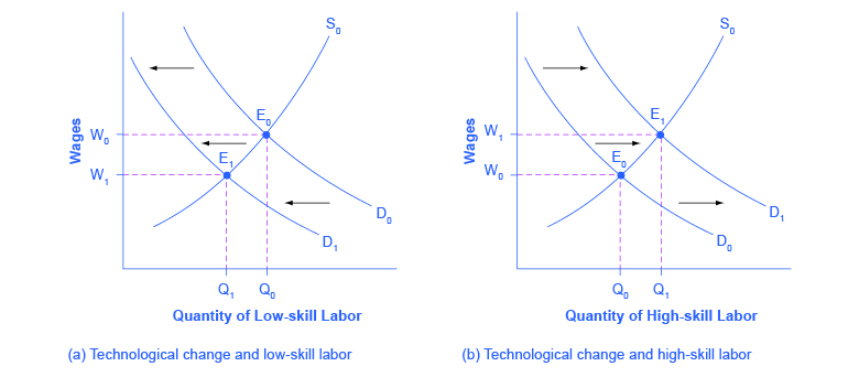
Figure 4.4a (Text Version)

Figure 4.4a contains two graphs: Graph A – Technological change and low-skill labour, Graph B – Technological change and high-skill labour.

Graph A: The graph has the vertical axis Wages (W) and Quantity of Low-Skill Labour (Q). The original supply curve (S₀) slopes upward from left to right. The original demand Curve (D₀) slopes downward from left to right. S₀ and D₀ intersect at the original equilibrium (E₀) at  price W₀ and quantity  Q₀ . D₀ shifts to the left and now intersects S₀ at a new equilibrium (E₁) at price W₁ and quantity  Q₁.

Graph B: The graph has the vertical axis Wages (W) and Quantity of High-Skill Labour (Q). The original supply curve (S₀) slopes upward from left to right. The original demand Curve (D₀) slopes downward from left to right. S₀ and D₀ intersect at the original equilibrium (E₀) at  price W₀ and quantity  Q₀ . D₁ shifts to the right and now intersects S₀ at a new equilibrium (E₁) at price W₁ and quantity  Q₁.

Step 2. Does the new technology affect the supply of labor from households or the demand for labor from firms?

Step 3. Will the new technology increase or decrease demand?

Step 4. Compare the new equilibrium price and quantity to the original equilibrium price.

Check your answers^[1]

So, the demand and supply model predicts that the new computer and communications technologies will raise the pay of high-skill workers but reduce the pay of low-skill workers. Indeed, from the 1970s to the mid-2000s, the wage gap widened between high-skill and low-skill labor. According to the National Center for Education Statistics, in 1980, for example, a college graduate earned about 30% more than a high school graduate with comparable job experience, but by 2012, a college graduate earned about 60% more than an otherwise comparable high school graduate. Many economists believe that the trend toward greater wage inequality across the U.S. economy was primarily caused by the new technologies.

Supply and Demand in Financial Markets

Now let’s examine how the theories of supply and demand also affect financial markets. Imagine that the U.S. economy became viewed as a less desirable place for foreign investors to put their money because of fears about the growth of the U.S. public debt. Using the four-step process for analyzing how changes in supply and demand affect equilibrium outcomes, how would increased U.S. public debt affect the equilibrium price and quantity for capital in U.S. financial markets?

The effect of growing U.S. debt: The four-step process

Step 1. Draw a diagram showing demand and supply for financial capital that represents the original scenario in which foreign investors are pouring money into the U.S. economy.

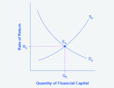
Figure 4.4b (Text Version)

The graph has a vertical axis is rate of return (R) and a horizontal axis Quantity if financial capital (Q). The demand curve (D₀) slopes downward from left to right  and the supply curve (S₀) slopes upward from left to right. The original equilibrium E₀ occurs where S₀ and D₀ intersect at interest rate R₀ and quantity of financial investment Q₀.

Figure 4.4b :Figure 4.4b shows a demand curve, D₀, and a supply curve, S₀, where the supply of capital includes the funds arriving from foreign investors. The original equilibrium E₀ occurs at interest rate R₀ and quantity of financial investment Q₀.The graph shows the demand for financial capital  and supply of financial capital into the U.S. financial markets by the foreign sector before the increase in uncertainty regarding U.S. public debt. The original equilibrium (E₀) occurs at an equilibrium rate of return (R₀) and the equilibrium quantity is at Q₀.

Step 2. Will the diminished confidence in the U.S. economy as a place to invest affect demand or supply of financial capital?

Step 3. Will supply increase or decrease? When the enthusiasm of foreign investors’ for investing their money in the U.S. economy diminishes, the supply of financial capital shifts to the left. Figure 4.4c shows the supply curve shift from S₀ to S1.

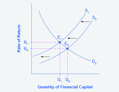
Figure 4.4c (Text Version)

Figure 4.4c uses Figure 2 as a base. The graph has a vertical axis is rate of return (R) and a horizontal axis Quantity if financial capital (Q). The original demand curve (D₀) slopes downward from left to right  and the original supply curve (S₀) slopes upward from left to right. The original equilibrium E₀ occurs where S₀ and D₀ intersect at interest rate R₀ and quantity of financial investment Q₀. The supply curve shift from S₀ to the left to S₁. The original demand curve (D₀) now intersects with the new supply curve (S₁)  at the new equilibrium E₁  interest rate R₁ and quantity of financial investment Q₁.

Figure 4.4c. The graph shows the demand for financial capital and supply of financial capital into the U.S. financial markets by the foreign sector before and after the increase in uncertainty regarding U.S. public debt. The original equilibrium (E₀) occurs at an equilibrium rate of return (R₀) and the equilibrium quantity is at Q₀.

Step 4. Compare the new equilibrium price and quantity to the original equilibrium price.

Check your answers^[2]

In a modern, developed economy, financial capital often moves invisibly through electronic transfers between one bank account and another. Yet these flows of funds can be analyzed with the same tools of demand and supply as markets for goods or labor.

Attribution

Except where otherwise noted, this chapter is adapted from “Labor and Financial Markets”  In Microeconomics  by Lumen Learning, licensed under CC BY 4.0. A derivative of “Labor and Financial Markets” In Principles of Macroeconomics by Steven A. Greenlaw and Timothy Taylor (OpenStax), licensed under CC BY 4.0.

Access for free at Principles of Macroeconomics