5.3 – Price Elasticity of Demand and Price Elasticity of Supply
Learning Objectives
- Calculate the price elasticity of demand
- Calculate the price elasticity of supply
Both the demand and supply curve show the relationship between price and the number of units demanded or supplied. Price elasticity is the ratio between the percentage change in the quantity demanded (Qd) or supplied (Qs) and the corresponding percent change in price. The price elasticity of demand is the percentage change in the quantity demanded of a good or service divided by the percentage change in the price. The price elasticity of supply is the percentage change in quantity supplied divided by the percentage change in price.
We can usefully divide elasticities into three broad categories: elastic, inelastic, and unitary. Because price and quantity demanded move in opposite directions, price elasticity of demand is always a negative number. Therefore, price elasticity of demand is usually reported as its absolute value, without a negative sign. The summary in Table 5.3a is assuming absolute values for price elasticity of demand. An elastic demand or elastic supply is one in which the elasticity is greater than one, indicating a high responsiveness to changes in price. Elasticities that are less than one indicate low responsiveness to price changes and correspond to inelastic demand or inelastic supply. Unitary elasticities indicate proportional responsiveness of either demand or supply, as Table 5.3a summarizes.
| If . . . | Then . . . | And It Is Called . . . |
|---|---|---|
| [latex]\% \text{change in quantity} > \% \text{change in price}[/latex] | [latex]\frac {\% \text{change in quantity}} {\% \text{change in price}}\ >1[/latex] | Elastic |
| [latex]\% \text{change in quantity} = \% \text{change in price}[/latex] | [latex]\frac {\% \text{change in quantity}} {\% \text{change in price}} = 1[/latex] | Unitary |
| [latex]\% \text{change in quantity} < \% \text{change in price}[/latex] | [latex]\frac{\% \text{change in quantity}} {\% \text{change in price}} <1[/latex] | Inelastic |
Link It Up
Before we delve into the details of elasticity, enjoy the article Super Bowl XLVIII Pricing: A Lesson In Demand Elasticity[New Tab] to learn about elasticity and ticket prices at the Super Bowl.
To calculate elasticity along a demand or supply curve economists use the average percent change in both quantity and price. This is called the Midpoint Method for Elasticity, and is represented in the following equations:
The advantage of the Midpoint Method is that one obtains the same elasticity between two price points whether there is a price increase or decrease. This is because the formula uses the same base (average quantity and average price) for both cases.
Calculating Price Elasticity of Demand
Let’s calculate the elasticity between points A and B and between points G and H as Figure 5.3a shows.
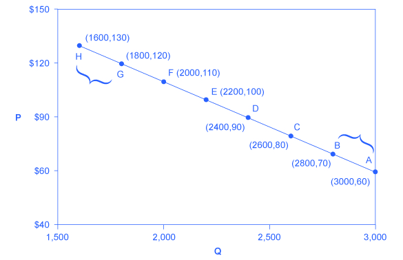
Figure 5.3a Calculating the Price Elasticity of Demand (Text Version)
| Points | Location on the graph (Quantity, Price) |
|---|---|
| A | (3000, 60) |
| B | (2800, 70) |
| C | (2600, 80) |
| D | (2400, 90) |
| E | (2200, 100) |
| F | (2000, 110) |
| G | (1800, 120) |
| H | (1600, 130) |
First, apply the formula to calculate the elasticity as price decreases from $70 at point B to $60 at point A:
Therefore, the elasticity of demand between these two points is 6.9%–15.4% 6.9%–15.4% which is 0.45, an amount smaller than one, showing that the demand is inelastic in this interval. Price elasticities of demand are always negative since price and quantity demanded always move in opposite directions (on the demand curve). By convention, we always talk about elasticities as positive numbers. Mathematically, we take the absolute value of the result. We will ignore this detail from now on, while remembering to interpret elasticities as positive numbers.
This means that, along the demand curve between point B and A, if the price changes by 1%, the quantity demanded will change by 0.45%. A change in the price will result in a smaller percentage change in the quantity demanded. For example, a 10% increase in the price will result in only a 4.5% decrease in quantity demanded. A 10% decrease in the price will result in only a 4.5% increase in the quantity demanded. Price elasticities of demand are negative numbers indicating that the demand curve is downward sloping, but we read them as absolute values. The following Work It Out feature will walk you through calculating the price elasticity of demand.
Work It Out
Finding the Price Elasticity of Demand
Calculate the price elasticity of demand using the data in Figure 5.3a for an increase in price from G to H. Has the elasticity increased or decreased?
Step 1. We know that:
Step 2. From the Midpoint Formula we know that:
Step 3. So we can use the values provided in the figure in each equation:
Step 4. Then, we can use those values to determine the price elasticity of demand:
[latex]{\normalsize\begin{array}{r @{{}={}} l} \: \text{Price Elasticity of Demand} =& \frac {\%\: \text{change in quantity}} {\%\: \text{change in price}}\\ =& \frac{-11.76}{8}\\=& 1.47\end{array}}[/latex]
Therefore, the elasticity of demand from G to is H 1.47. The magnitude of the elasticity has increased (in absolute value) as we moved up along the demand curve from points A to B. Recall that the elasticity between these two points was 0.45. Demand was inelastic between points A and B and elastic between points G and H. This shows us that price elasticity of demand changes at different points along a straight-line demand curve.
Calculating the Price Elasticity of Supply
Assume that an apartment rents for $650 per month and at that price the landlord rents 10,000 units are rented as Figure 5.3b shows. When the price increases to $700 per month, the landlord supplies 13,000 units into the market. By what percentage does apartment supply increase? What is the price sensitivity?
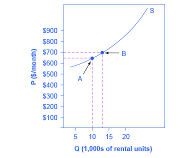
Figure 5.3b Price Elasticity of Supply (Text Version)
The graph shows an upward sloping line that represents the supply of apartment rentals. The vertical axis is Price ($/month) and the horizontal axis is Quantity (1,000s of rental units). The supply curve (S) has a concave upward slope running from left to right. Point A (10, 000 rental units, $650) and Point B (11, 500 rental units, $700) occur along the line.
[latex]\begin{array}{r @{{}={}} l}\%\;change\;in\;quantity= & \frac { 13,000-10,00}{ (13,000-10,00)/2 }\times 100 \\[1em] = & \frac { 3,000 }{11,500} \times 100 \\[1em] & = 26.1\\[1em] \%\;change\;in\;price = & \frac { 700-650}{ (700+650)/2} \times 100 \\[1em] =& \frac {50}{675}\times 100\\[1em] =& 7.4\\[1em] Price\;Elasticity\;of\;Demand = & \frac {26.1\%}{7.4\%}\\[1em]=&3.53 \end{array}[/latex]
Again, as with the elasticity of demand, the elasticity of supply is not followed by any units. Elasticity is a ratio of one percentage change to another percentage change—nothing more—and we read it as an absolute value. In this case, a 1% rise in price causes an increase in quantity supplied of 3.5%. The greater than one elasticity of supply means that the percentage change in quantity supplied will be greater than a one percent price change. If you’re starting to wonder if the concept of slope fits into this calculation, read the following Clear It Up box.
Clear It Up
Is the elasticity the slope?
It is a common mistake to confuse the slope of either the supply or demand curve with its elasticity. The slope is the rate of change in units along the curve, or the rise/run (change in y over the change in x). For example, in Figure 5.3a, at each point shown on the demand curve, price drops by $10 and the number of units demanded increases by 200 compared to the point to its left. The slope is –10/200 along the entire demand curve and does not change. The price elasticity, however, changes along the curve. Elasticity between points A and B was 0.45 and increased to 1.47 between points G and H. Elasticity is the percentage change, which is a different calculation from the slope and has a different meaning.
When we are at the upper end of a demand curve, where price is high and the quantity demanded is low, a small change in the quantity demanded, even in, say, one unit, is pretty big in percentage terms. A change in price of, say, a dollar, is going to be much less important in percentage terms than it would have been at the bottom of the demand curve. Likewise, at the bottom of the demand curve, that one unit change when the quantity demanded is high will be small as a percentage.
Thus, at one end of the demand curve, where we have a large percentage change in quantity demanded over a small percentage change in price, the elasticity value would be high, or demand would be relatively elastic. Even with the same change in the price and the same change in the quantity demanded, at the other end of the demand curve the quantity is much higher, and the price is much lower, so the percentage change in quantity demanded is smaller and the percentage change in price is much higher. That means at the bottom of the curve we’d have a small numerator over a large denominator, so the elasticity measure would be much lower, or inelastic.
As we move along the demand curve, the values for quantity and price go up or down, depending on which way we are moving, so the percentages for, say, a $1 difference in price or a one unit difference in quantity, will change as well, which means the ratios of those percentages and hence the elasticity will change.
Key Concepts and Summary
Price elasticity measures the responsiveness of the quantity demanded or supplied of a good to a change in its price. We compute it as the percentage change in quantity demanded (or supplied) divided by the percentage change in price. We can describe elasticity as elastic (or very responsive), unit elastic, or inelastic (not very responsive). Elastic demand or supply curves indicate that quantity demanded or supplied respond to price changes in a greater than proportional manner. An inelastic demand or supply curve is one where a given percentage change in price will cause a smaller percentage change in quantity demanded or supplied. A unitary elasticity means that a given percentage change in price leads to an equal percentage change in quantity demanded or supplied.
Attribution
Except where otherwise noted, this chapter is adapted from “Price Elasticity of Demand and Price Elasticity of Supply” and “Key Concepts and Summary” In Principles of Microeconomics 2e (OpenStax) by Steven A. Greenlaw & David Shapiro, licensed under CC BY 4.0.
Access for free at Principles of Microeconomics 2e
Original Source Chapter References
Abkowitz, A. “How Netflix got started: Netflix founder and CEO Reed Hastings tells Fortune how he got the idea for the DVD-by-mail service that now has more than eight million customers.” CNN Money. Last Modified January 28, 2009. http://archive.fortune.com/2009/01/27/news/newsmakers/hastings_netflix.fortune/index.htm.
Associated Press (a). ”Analyst: Coinstar gains from Netflix pricing moves.” Boston Globe Media Partners, LLC. Accessed June 24, 2013. http://www.boston.com/business/articles/2011/10/12/analyst_coinstar_gains_from_netflix_pricing_moves/.
Associated Press (b). “Netflix loses 800,000 US subscribers in tough 3Q.” ABC Inc. Accessed June 24, 2013. http://abclocal.go.com/wpvi/story?section=news/business&id=8403368
Baumgardner, James. 2014. “Presentation on Raising the Excise Tax on Cigarettes: Effects on Health and the Federal Budget.” Congressional Budget Office. Accessed March 27, 2015. http://www.cbo.gov/sites/default/files/45214-ICA_Presentation.pdf.
Funding Universe. 2015. “Netflix, Inc. History.” Accessed March 11, 2015. http://www.fundinguniverse.com/company-histories/netflix-inc-history/.
Laporte, Nicole. “A tale of two Netflix.” Fast Company 177 (July 2013) 31-32. Accessed December 3 2013. http://www.fastcompany-digital.com/fastcompany/20130708?pg=33#pg33
Liedtke, Michael, The Associated Press. “Investors bash Netflix stock after slower growth forecast – fee hikes expected to take toll on subscribers most likely to shun costly bundled Net, DVD service.” The Seattle Times. Accessed June 24, 2013 from NewsBank on-line database (Access World News).
Netflix, Inc. 2013. “A Quick Update On Our Streaming Plans And Prices.” Netflix (blog). Accessed March 11, 2015. http://blog.netflix.com/2014/05/a-quick-update-on-our-streaming-plans.html.
Organization for Economic Co-Operation and Development (OECC). n.d. “Average annual hours actually worked per worker.” Accessed March 11, 2015. https://stats.oecd.org/Index.aspx?DataSetCode=ANHRS.
Savitz, Eric. “Netflix Warns DVD Subs Eroding; Q4 View Weak; Losses Ahead; Shrs Plunge.” Forbes.com, 2011. Accessed December 3, 2013. http://www.forbes.com/sites/ericsavitz/2011/10/24/netflix-q3-top-ests-but-shares-hit-by-weak-q4-outlook/.
Statistica.com. 2014. “Coffee Export Volumes Worldwide in November 2014, by Leading Countries (in 60-kilo sacks).” Accessed March 27, 2015. http://www.statista.com/statistics/268135/ranking-of-coffee-exporting-countries/.
Stone, Marcie. “Netflix responds to customers angry with price hike; Netflix stock falls 9%.” News & Politics Examiner, 2011. Clarity Digital Group. Accessed June 24, 2013. http://www.examiner.com/article/netflix-responds-to-customers-angry-with-price-hike-netflix-stock-falls-9.
Weinman, J. (2012). Die hard, hardly dying. Maclean’s, 125(18), 44.
The World Bank Group. 2015. “Gross Savings (% of GDP).” Accessed March 11, 2015. http://data.worldbank.org/indicator/NY.GNS.ICTR.ZS.
Yahoo Finance. Retrieved from http://finance.yahoo.com/q?s=NFLX
Media Attributions
- Figure 5.2 Calculating the Price Elasticity of Demand © Steven A. Greenlaw & David Shapiro (OpenStax) is licensed under a CC BY (Attribution) license
- Figure 5.3 Price Elasticity of Supply © Steven A. Greenlaw & David Shapiro (OpenStax)
The relationship between the percent change in price resulting in a corresponding percentage change in the quantity demanded or supplied
