9.2 Statistical Inference for Two Population Means with Known Population Standard Deviations
LEARNING OBJECTIVES
- Construct and interpret a confidence interval for two population means with known population standard deviations.
- Conduct and interpret hypothesis tests for two population means with known population standard deviations.
The comparison of two population means is very common. Often, we want to find out if the two populations under study have the same mean or if there is some difference in the two population means. The approach we take when studying two population means depends on whether the samples are independent or matched. In the case where the samples are independent, we also have to contend with whether or not we know the population standard deviations.
Two populations are independent if the sample taken from population 1 is not related in anyway to the sample taken from population 2. In this situation, any relationship between the samples or populations is entirely coincidental.
Throughout this section, we will use subscripts to identify the values for the means, sample sizes, and standard deviations for the two populations:
| Symbol for: | Population 1 | Population 2 |
| Population Mean | [latex]\mu_1[/latex] | [latex]\mu_2[/latex] |
| Population Standard Deviation | [latex]\sigma_1[/latex] | [latex]\sigma_2[/latex] |
| Sample Size | [latex]n_1[/latex] | [latex]n_2[/latex] |
| Sample Mean | [latex]\overline{x}_1[/latex] | [latex]\overline{x}_2[/latex] |
| Sample Standard Deviation | [latex]s_1[/latex] | [latex]s_2[/latex] |
In order to construct a confidence interval or conduct a hypothesis test on the difference in two population means ([latex]\mu_1-\mu_2[/latex]), we need to use the distribution of the difference in the sample means [latex]\overline{x}_1-\overline{x}_2[/latex]:
- The mean of the distribution of the difference in the sample means is [latex]\displaystyle{\mu_{\overline{x}_1-\overline{x}_2}}=\mu_1-\mu_2[/latex].
- The standard deviation of the distribution of the difference in the sample means is:
[latex]\displaystyle{\sigma_{\overline{x}_1-\overline{x}_2}=\sqrt{\frac{\sigma_1^2}{n_1}+\frac{\sigma_2^2}{n_2}}}[/latex].
- The distribution of the difference in the sample means is normal if one of the following is true:
- Both populations are normally distributed.
- The sample sizes are large enough ([latex]n_1 \geq 30[/latex] and [latex]n_2 \geq 30[/latex]).
- Assuming the distribution of the difference of the sample means is normal, the [latex]z[/latex]-score is
[latex]\displaystyle{z=\frac{(\overline{x}_1-\overline{x}_2)-(\mu_1-\mu_2)}{\sqrt{\frac{\sigma_1^2}{n_1}+\frac{\sigma_2^2}{n_2}}}}[/latex]
Constructing a Confidence Interval for the Difference in Two Population Means with Known Population Standard Deviation
Suppose a sample of size [latex]n_1[/latex] with sample mean [latex]\overline{x}_1[/latex] is taken from population 1 and a sample of size [latex]n_2[/latex] with sample mean [latex]\overline{x}_2[/latex] is taken from population 2 where the populations are independent and the population standard deviations, [latex]\sigma_1[/latex] and [latex]\sigma_2[/latex], are known. The limits for the confidence interval with confidence level [latex]C[/latex] for the difference in the population means [latex]\displaystyle{\mu_1-\mu_2}[/latex] are:
[latex]\begin{eqnarray*}\\\text{Lower Limit}&=&\overline{x}_1-\overline{x}_2-z\times\sqrt{\frac{\sigma^2_1}{n_1}+\frac{\sigma^2_2}{n_2}}\\\\\text{Upper Limit}&=&\overline{x}_1-\overline{x}_2+z\times\sqrt{\frac{\sigma^2_1}{n_1}+\frac{\sigma^2_2}{n_2}}\\\end{eqnarray*}[/latex]
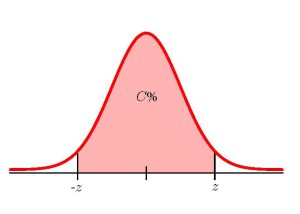
where [latex]z[/latex] is the positive [latex]z[/latex]-score of the standard normal distribution so that the area under the curve in between [latex]-z[/latex] and [latex]z[/latex] is [latex]C\%[/latex].
NOTE
In order to construct the confidence interval for the difference in two population means with independent samples, we need to check that the distribution of the difference in the sample means follows a normal distribution. This means that we need to check that either the populations are normal or that the sample sizes are large enough (greater than or equal to 30).
CALCULATING THE [latex]{\color{white}{z}}[/latex]-SCORE FOR A CONFIDENCE INTERVAL IN EXCEL
To find the [latex]z[/latex]-score to construct a confidence interval with confidence level [latex]C[/latex], use the norm.s.inv(area to the left of z) function.
- For area to the left of z, enter the entire area to the left of the [latex]z[/latex]-score you are trying to find. For a confidence interval, the area to the left of [latex]z[/latex] is [latex]\displaystyle{C+\frac{1-C}{2}}[/latex].
The output from the norm.s.inv function is the value of the [latex]z[/latex]-score needed to construct the confidence interval.
NOTE
The norm.s.inv function requires that we enter the entire area to the left of the unknown [latex]z[/latex]-score. This area includes the confidence level (the area in the middle of the distribution) plus the remaining area in the left tail.
EXAMPLE
A consumer advocacy group wants to study consumer satisfaction with their shopping experience at the country's two biggest retailers. The group surveyed consumers and asked them to rate one of the retailers in a number of different categories. An overall satisfaction score out of 100 summarized the responses for each consumer sampled. In a sample of 35 consumers for retailer A, the average overall satisfaction score was 79. In a sample of 30 consumers for retailer B, the average overall satisfaction score was 71. Based on prior experience with the satisfaction rating scale, the population standard deviation for retailer A is assumed to be 10 and the population standard deviation for retailer B is assumed to be 12.
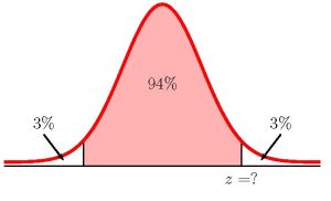
- Construct a 94% confidence interval for the difference in the mean satisfaction score for the two retailers.
- Interpret the confidence interval found in part 1.
- Is there evidence to suggest that the mean satisfaction score for retailer A is greater than the mean satisfaction score for retailer B? Explain.
Solution:
- Let retailer A be population 1 and retailer B be population 2. These populations are independent because there is no relationship between the consumers sampled for each retailer. From the question, we have the following information:
Retailer A Retailer B [latex]n_1=35[/latex] [latex]n_2=30[/latex] [latex]\overline{x}_1=79[/latex] [latex]\overline{x}_2=71[/latex] [latex]\sigma_1=10[/latex] [latex]\sigma_2=12[/latex] The normal distribution applies because the sample sizes are both greater than or equal to 30.
To find the confidence interval, we need to find the [latex]z[/latex]-score for the 94% confidence interval. This means that we need to find the [latex]z[/latex]-score so that the entire area to the left of [latex]z[/latex] is [latex]\displaystyle{0.94+\frac{1-0.94}{2}=0.97}[/latex].
Function norm.s.inv Answer Field 1 0.97 1.8807... So [latex]z=1.8807...[/latex]. The 94% confidence interval is
[latex]\begin{eqnarray*}\\\text{Lower Limit}&=&\overline{x}_1-\overline{x}_2-z\times\sqrt{\frac{\sigma_1^2}{n_1}+\frac{\sigma_2^2}{n_2}}\\&=&79-71-1.8807... \times\sqrt{\frac{10^2}{35}+\frac{12^2}{30}}\\&=&2.796 \\\\\text{Upper Limit}& = &\overline{x}_1-\overline{x}_2+z\times\sqrt{\frac{\sigma_1^2}{n_1}+\frac{\sigma_2^2}{n_2}}\\&=&79-71+1.8807...\times\sqrt{\frac{10^2}{35}+\frac{12^2}{30}}\\&=&13.204\\\\\end{eqnarray*}[/latex]
- We are 94% confident that the difference in the mean satisfaction score for the two retailers is between 2.796 and 13.204.
- Because 0 is outside the confidence interval and both limits are positive, it suggests that the difference in the means [latex]\displaystyle{\mu_1-\mu_2}[/latex] is greater than 0. That is, [latex]\displaystyle{\mu_1-\mu_2 \gt 0}[/latex] ([latex]\mu_1 \gt \mu_2[/latex]). This suggests that the mean for population 1 (retailer A) is greater than the mean for population 2 (retailer B). So the mean satisfaction score for retailer A is greater than the mean satisfaction score for retailer B.
NOTES
- When calculating the limits for the confidence interval keep all of the decimals in the [latex]z[/latex]-score and other values throughout the calculation. This will ensure that there is no round-off error in the answers. You can use Excel to do the calculation of the limits, clicking on the cells containing the [latex]z[/latex]-score or any other values, to ensure that all of the decimal places are used in the calculation.
- When writing down the interpretation of the confidence interval, make sure to include the confidence level, the actual difference in the population means captured by the confidence interval (i.e. be specific to the context of the question), and appropriate units for the limits.
Steps to Conduct a Hypothesis Test for the Difference in Two Independent Population Means with Known Population Standard Deviations
- Write down the null hypothesis that there is no difference in the population means:
[latex]\begin{eqnarray*}\\H_0:&& \mu_1-\mu_2=0\end{eqnarray*}[/latex]
The null hypothesis is always the claim that the two population means are equal ([latex]\mu_1=\mu_2[/latex]).
- Write down the alternative hypotheses in terms of the difference in the population means. The alternative hypothesis will be one of the following:
[latex]\begin{eqnarray*}\\H_a:\mu_1-\mu_2<0&&(\mu_1\lt\mu_2)\\H_a:\mu_1-\mu_2>0&&(\mu_1\gt\mu_2)\\H_a:\mu_1-\mu_2\neq 0&&(\mu_1\neq\mu_2)\\\\\end{eqnarray*}[/latex]
- Use the form of the alternative hypothesis to determine if the test is left-tailed, right-tailed, or two-tailed.
- Collect the sample information for the test and identify the significance level.
- Assuming the population standard deviations are known, use the normal distribution to find the p-value (the area in the corresponding tail) for the test. The [latex]z[/latex]-score is
[latex]\begin{eqnarray*}z & = & \frac{(\overline{x}_1-\overline{x}_2)-(\mu_1-\mu_2)}{\sqrt{\frac{\sigma_1^2}{n_1}+\frac{\sigma_2^2}{n_2}}} \\ \\ \end{eqnarray*}[/latex]
- Compare the p-value to the significance level and state the outcome of the test:
- If p-value[latex]\leq \alpha[/latex], reject [latex]H_0[/latex] in favour of [latex]H_a[/latex].
- The results of the sample data are significant. There is sufficient evidence to conclude that the null hypothesis [latex]H_0[/latex] is an incorrect belief and that the alternative hypothesis [latex]H_a[/latex] is most likely correct.
- If p-value[latex]\gt \alpha[/latex], do not reject [latex]H_0[/latex].
- The results of the sample data are not significant. There is not sufficient evidence to conclude that the alternative hypothesis [latex]H_a[/latex] may be correct.
- If p-value[latex]\leq \alpha[/latex], reject [latex]H_0[/latex] in favour of [latex]H_a[/latex].
- Write down a concluding sentence specific to the context of the question.
USING EXCEL TO CALCULE THE P-VALUE FOR A HYPOTHESIS TEST ON TWO INDEPENDENT POPULATION MEANS WITH KNOWN POPULATION STANDARD DEVIATIONS
Assuming that the population standard deviations are known, the p-value for a hypothesis test on the difference in two independent population means is the area in the tail(s) of the normal distribution.
The p-value is the area in the tail(s) of a normal distribution, so the norm.dist(x,[latex]\mu[/latex],[latex]\sigma[/latex],logic operator) function can be used to calculate the p-value.
- For x, enter the value for [latex]\overline{x}_1-\overline{x}_2[/latex].
- For [latex]\mu[/latex], enter the 0, the value of [latex]\mu_1-\mu_2[/latex] from the null hypothesis. This is the mean of the distribution of the differences in the sample means.
- For [latex]\sigma[/latex], enter the value of [latex]\displaystyle{\sigma_{\overline{x}_1-\overline{x}_2}=\sqrt{\frac{\sigma_1^2}{n_1}+\frac{\sigma_2^2}{n_2}}}[/latex], the standard deviation of the distribution of the differences in the sample mean.
- For the logic operator, enter true. Note: Because we are calculating the area under the curve, we always enter true for the logic operator.
As with the previous chapter, use the appropriate technique with the norm.dist function to find the area in the left-tail, the area in the right-tail or the sum of the area in tails.
EXAMPLE
A floor cleaning company has been using Wax 1 to wax floors for a long time. A new floor wax, Wax 2, has recently come on the market with the claim that it is longer lasting than Wax 1. The company wants to investigate this claim. The company waxed a sample of 20 floors with Wax 1 and found the average number of months the wax lasted was 2.7 months. The company waxed a sample of 20 floors with Wax 2 and found the average number of months the wax lasted was 2.9 months. Based on previous information, the standard deviation for the length of time Wax 1 lasts is 0.33 months and the standard deviation for the length of time Wax 2 lasts is 0.36 months. Both populations have normal distributions. At the 5% significance level, test if Wax 2 lasts longer, on average, than Wax 1.
Solution:
Let Wax 1 be population 1 and Wax 2 be population 2. These populations are independent because there is no relationship between the length of time each type of wax lasts. From the question, we have the following information:
| Wax 1 | Wax 2 |
| [latex]n_1=20[/latex] | [latex]n_2=20[/latex] |
| [latex]\overline{x}_1=2.7[/latex] | [latex]\overline{x}_2=2.9[/latex] |
| [latex]\sigma_1=0.33[/latex] | [latex]\sigma_2=0.36[/latex] |
Hypotheses:
[latex]\begin{eqnarray*}H_0:&&\mu_1-\mu_2=0\\H_a:&&\mu_1-\mu_2 \lt 0 \end{eqnarray*}[/latex]
p-value:
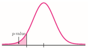
This is a test on a the difference in two population means where the population standard deviation are known. So we use a normal distribution to calculate the p-value. Because the alternative hypothesis is a [latex]\lt[/latex], the p-value is the area in the left-tail of the distribution.
| Function | norm.dist | Answer |
| Field 1 | 2.7-2.9 | 0.0335 |
| Field 2 | 0 | |
| Field 3 | sqrt(0.33^2/20+0.36^2/20) | |
| Field 4 | true |
So the p-value[latex]=0.0335[/latex].
Conclusion:
Because p-value[latex]=0.0335 \lt 0.05=\alpha[/latex], we reject the null hypothesis in favour of the alternative hypothesis. At the 5% significance level there is enough evidence to suggest that Wax 2 lasts longer than Wax 1.
NOTES
- The null hypothesis [latex]\mu_1-\mu_2=0[/latex] is the claim that the mean number of months for Wax 1 equals the mean number of months for Wax 2. That is, the two types of waxes have the same mean.
- The alternative hypothesis [latex]\mu_1 -\mu_2 \lt 0[/latex] is the claim that the mean for Wax 1 is less than the mean for Wax 2 ([latex]\mu_1 \lt \mu_2[/latex]). This is the same as saying that the mean for Wax 2 is larger than the mean for Wax 1.
- The p-value is the area in the left tail of the normal distribution. In the calculation of the p-value:
- The function is norm.dist because we are finding the area in the left tail of a normal distribution.
- Field 1 is the value of [latex]\overline{x}_1-\overline{x}_2=2.7-2.9[/latex]
- Field 2 is 0, the value of [latex]\mu_1-\mu_2[/latex] from the null hypothesis. Remember, we run the test assuming the null hypothesis is true, so that means we assume [latex]\mu_1-\mu_2=0[/latex].
- Field 3 is the standard deviation for the difference in the sample means [latex]\displaystyle{\sqrt{\frac{\sigma_1^2}{n_1}+\frac{\sigma_2^2}{n_2}}=\sqrt{\frac{0.33^2}{20}+\frac{0.36^2}{20}}}[/latex].
- The p-value of 0.0335 is a small probability compared to the significance level, and so is unlikely to happen assuming the null hypothesis is true. This suggests that the assumption that the null hypothesis is true is most likely incorrect, and so the conclusion of the test is to reject the null hypothesis in favour of the alternative hypothesis. In other words, the mean number of months for Wax 1 is less than the mean number of months for Wax 2. For the company this suggests that they should switch to Wax 2 because of it is longer lasting than Wax 1.
EXAMPLE
A consumer advocacy group wants to compare the revolutions per minute (RPM) for two different engines. The group believes that Engine A has a higher average RPM than Engine B. In a sample of 40 Engine A's, the sample mean number of RPMs was 1550. In a sample of 30 Engine B's, the sample mean number of RPMs was 1500. Based on previous information, the standard deviation for the RPMs for Engine A is 75 and the standard deviation for Engine B is 65. At the 1% significance level, is the average RPM for Engine A higher than for Engine B?
Solution:
Let Engine A be population 1 and Engine B be population 2. These populations are independent because there is no relationship between the RPMs for the two engines. From the questions, we have the following information:
| Engine A | Engine B |
| [latex]n_1=40[/latex] | [latex]n_2=30[/latex] |
| [latex]\overline{x}_1=1550[/latex] | [latex]\overline{x}_2=1500[/latex] |
| [latex]\sigma_1=75[/latex] | [latex]\sigma_2=65[/latex] |
Hypotheses:
[latex]\begin{eqnarray*}H_0:&&\mu_1-\mu_2=0\\H_a:&&\mu_1-\mu_2\gt 0\end{eqnarray*}[/latex]
p-value:
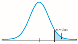
This is a test on a the difference in two population means where the population standard deviation are known. So we use a normal distribution to calculate the p-value. Because the alternative hypothesis is a [latex]\gt[/latex], the p-value is the area in the right tail of the distribution.
| Function | 1-norm.dist | Answer |
| Field 1 | 1550-1500 | 0.0014 |
| Field 2 | 0 | |
| Field 3 | sqrt(75^2/40+65^2/30) | |
| Field 4 | true |
So the p-value[latex]=0.0014[/latex].
Conclusion:
Because p-value[latex]=0.0014 \lt 0.01=\alpha[/latex], we reject the null hypothesis in favour of the alternative hypothesis. At the 1% significance level there is enough evidence to suggest that the average RPM for Engine A is higher than for Engine B.
NOTES
- The null hypothesis [latex]\mu_1-\mu_2=0[/latex] is the claim that the mean RPM for Engine A equals the mean RPM for Engine B. That is, the two engines have the same average RPM.
- The alternative hypothesis [latex]\mu_1 -\mu_2 \gt 0[/latex] is the claim that the mean RPM for Engine A is greater than the mean RPM for Engine B ([latex]\mu_1 \gt \mu_2[/latex]).
- The p-value is the area in the right tail of the normal distribution. In the calculation of the p-value:
- The function is 1-norm.dist because we are finding the area in the right tail of a normal distribution.
- Field 1 is the value of [latex]\overline{x}_1-\overline{x}_2=1550-1500[/latex]
- Field 2 is 0, the value of [latex]\mu_1-\mu_2[/latex] from the null hypothesis. Remember, we run the test assuming the null hypothesis is true, so that means we assume [latex]\mu_1-\mu_2=0[/latex].
- Field 3 is the standard deviation for the difference in the sample means [latex]\displaystyle{\sqrt{\frac{\sigma_1^2}{n_1}+\frac{\sigma_2^2}{n_2}}=\sqrt{\frac{75^2}{40}+\frac{65^2}{30}}}[/latex].
- The p-value of 0.0014 is a small probability compared to the significance level, and so is unlikely to happen assuming the null hypothesis is true. This suggests that the assumption that the null hypothesis is true is most likely incorrect, and so the conclusion of the test is to reject the null hypothesis in favour of the alternative hypothesis. In other words, the mean RPM for Engine A is greater than the mean RPM for Engine B, just as the consumer advocacy group claimed.
EXAMPLE
The student union at a local college owns two coffee shops on campus: The Study Cafe and Coffee&Books. The student union wants to find out if there is a difference the average amount students spend per transaction at each of the coffee shops. In a sample of 65 transactions at the Study Cafe, the average amount spent was $9.40. In a sample of 50 transactions at Coffee&Books, the average amount spent was $10.15. Based on previous information, the standard deviation for the amount spent at the Study Cafe is $1.35 and the standard deviation for Coffee&Books B is $2.70. At the 5% significance level, is there a difference in the average amount spent per transaction at the two coffee shops?
Solution:
Let the Study Cafe be population 1 and Coffee&Books be population 2. These populations are independent because there is no relationship between the amount spent at each coffee shop. From the question, we have the following information:
| The Study Cafe | Coffee&Books |
| [latex]n_1=65[/latex] | [latex]n_2=50[/latex] |
| [latex]\overline{x}_1=9.40[/latex] | [latex]\overline{x}_2=10.15[/latex] |
| [latex]\sigma_1=1.35[/latex] | [latex]\sigma_2=2.70[/latex] |
Hypotheses:
[latex]\begin{eqnarray*}H_0:&&\mu_1-\mu_2=0\\H_a:&&\mu_1-\mu_2\neq 0\end{eqnarray*}[/latex]
p-value:
This is a test on a the difference in two population means where the population standard deviation are known. So we use a normal distribution to calculate the p-value. Because the alternative hypothesis is a [latex]\neq[/latex], the p-value is the sum of the area in the two tails of the distribution.
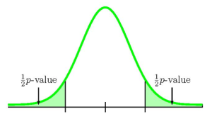
We need to know if the sample information relates to the left or right tail because that will determine how we calculate out the area of that tail using the normal distribution. In this case, the [latex]\overline{x}_1 \lt \overline{x}_2[/latex] ([latex]9.4 \lt 10.15[/latex]), so the sample information relates to the left tail of the normal distribution. This means that we will calculate out the area in the left tail using norm.dist. However, this is a two-tailed test where the p-value is the sum of the area in the two tails and the area in the left tail is only one half of the p-value. The area in the left tail equals the area in the right tail and the p-value is the sum of these two areas.
| Function | norm.dist | Answer |
| Field 1 | 9.40-10.15 | 0.0360 |
| Field 2 | 0 | |
| Field 3 | sqrt(1.35^2/65+2.7^2/50) | |
| Field 4 | true |
So the area in the left tail is 0.0360, which means [latex]\frac{1}{2}[/latex](p-value)[latex]=0.0360[/latex]. This is also the area in the right tail, so
p-value[latex]=0.0360+0.0360=0.0720[/latex]
Conclusion:
Because p-value[latex]=0.0720 \gt 0.05=\alpha[/latex], we do not reject the null hypothesis. At the 5% significance level there is not enough evidence to suggest that there is a difference in the average amount spent at the two coffee shops.
NOTES
- The null hypothesis [latex]\mu_1-\mu_2=0[/latex] is the claim that the mean amount spent at the Study Cafe equals the mean amount spent at Coffee&Books. That is, the average amount spent is the same at both coffee shops.
- The alternative hypothesis [latex]\mu_1 -\mu_2 \neq 0[/latex] is the claim that the mean amount spent at the Study Cafe is different than the mean amount spent at Coffee&Books ([latex]\mu_1 \neq \mu_2[/latex]).
- In a two-tailed hypothesis test that uses the normal distribution, we will only have sample information relating to one of the two tails. We must determine which of the tails the sample information belongs to, and then calculate out the area in that tail. The area in each tail represents exactly half of the p-value, so the p-value is the sum of the areas in the two tails.
- If the sample mean [latex]\overline{x}_1[/latex] is less than the sample mean [latex]\overline{x}_2[/latex] ([latex]\overline{x}_1 \lt \overline{x}_2[/latex]), the sample information belongs to the left tail.
- We use norm.dist([latex]\overline{x}_1-\overline{x}_2[/latex],[latex]0[/latex],[latex]\sqrt{\frac{\sigma_1^2}{n_1}+\frac{\sigma_2^2}{n_2}}[/latex],true) to find the area in the left tail. The area in the right tail equals the area in the left tail, so we can find the p-value by adding the output from this function to itself.
- If the sample mean [latex]\overline{x}_1[/latex] is greater than the sample mean [latex]\overline{x}_2[/latex] ([latex]\overline{x}_1 \gt \overline{x}_2[/latex]), the sample information belongs to the right tail.
- We use 1-norm.dist([latex]\overline{x}_1-\overline{x}_2[/latex],[latex]0[/latex],[latex]\sqrt{\frac{\sigma_1^2}{n_1}+\frac{\sigma_2^2}{n_2}}[/latex],true) to find the area in the right tail. The area in the left tail equals the area in the right tail, so we can find the p-value by adding the output from this function to itself.
- If the sample mean [latex]\overline{x}_1[/latex] is less than the sample mean [latex]\overline{x}_2[/latex] ([latex]\overline{x}_1 \lt \overline{x}_2[/latex]), the sample information belongs to the left tail.
- The p-value of 0.0720 is a large probability compared to the significance level, and so is likely to happen assuming the null hypothesis is true. This suggests that the assumption that the null hypothesis is true is most likely correct, and so the conclusion of the test is to not reject the null hypothesis. In other words, the mean amount spent at the Study Cafe equals the mean amount spent at Coffee&Books.
Watch this video: Confidence Intervals for Two Population Means, Sigma Known by ExcelIsFun [9:52]
Watch this video: Hypothesis Testing for Two Population Means, Sigma Known by ExcelIsFun [16:47]
Concept Review
The general form of a confidence interval for the difference in two independent population means with known population standard deviations is
[latex]\begin{eqnarray*} \\ \mbox{Lower Limit} & = & \overline{x}_1-\overline{x}_2-z \times \sqrt{\frac{\sigma^2_1}{n_1}+\frac{\sigma^2_2}{n_2}} \\ \\ \mbox{Upper Limit} & = & \overline{x}_1-\overline{x}_2+z \times \sqrt{\frac{\sigma^2_1}{n_1}+\frac{\sigma^2_2}{n_2}} \\ \\ \end{eqnarray*}[/latex]
where [latex]z[/latex] is the positive [latex]z[/latex]-score of the standard normal distribution so the area under the normal distribution in between [latex]-z[/latex] and [latex]z[/latex] is [latex]C[/latex].
The hypothesis test for the difference in two independent population means with known population standard deviations is a well established process:
-
- Write down the null and alternative hypotheses in terms of the differences in the population means [latex]\mu_1-\mu_2[/latex].
- Use the form of the alternative hypothesis to determine if the test is left-tailed, right-tailed, or two-tailed.
- Collect the sample information for the test and identify the significance level.
- Find the p-value (the area in the corresponding tail) for the test using the normal distribution. Because the population standard deviations are known, we use the normal distribution to find the p-value.
- Compare the p-value to the significance level and state the outcome of the test.
- Write down a concluding sentence specific to the context of the question.
Attribution
"10.2 Two Population Means with Known Standard Deviations" in Introductory Statistics by OpenStax is licensed under a Creative Commons Attribution 4.0 International License.

