5.2 Probability Distribution of a Continuous Random Variable
LEARNING OBJECTIONS
- Recognize and understand continuous probability distributions.
For a continuous random variable, the curve of the probability distribution is denoted by the function [latex]f(x)[/latex]. The function [latex]f(x)[/latex] is called a probability density function and [latex]f(x)[/latex] produces the curve of the distribution. The function [latex]f(x)[/latex] is defined so that the area between it and the [latex]x[/latex]-axis is equal to a probability.
NOTE
The probability density function [latex]f(x)[/latex] does NOT give us probabilities associated with the continuous random variable. The function [latex]f(x)[/latex] produces the graph of the distribution and the area under this graph corresponds to the probability.
Properties of a continuous probability distribution include:
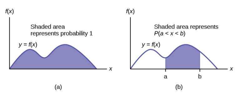
- The total area under the curve of the distribution is 1.
- The probability that the continuous random variable takes on a value in between [latex]c[/latex] and [latex]d[/latex] is the area under the curve of the distribution in between [latex]x=c[/latex] and [latex]x=d[/latex].
- The probability that the continuous random variable exactly equals a particular number ([latex]P(x=c)[/latex]) is 0.
EXAMPLE
Consider the probability density function [latex]f(x)=\displaystyle\frac{1}{20}[/latex] for [latex]0 \leq x \leq 20[/latex].
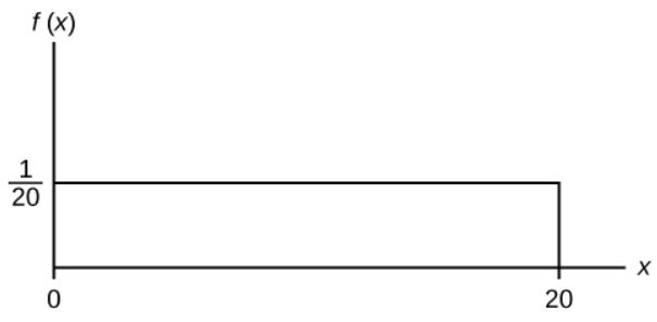
The graph of [latex]\displaystyle{f(x)=\frac{1}{20}}[/latex] with [latex]0 \leq x \leq 20[/latex] is a horizontal line segment from [latex]x=0[/latex] to [latex]x=20[/latex]. Note that the total area under the curve of [latex]f(x)[/latex], above the [latex]x[/latex]-axis, from [latex]x=0[/latex] to [latex]x=20[/latex] is
[latex]\displaystyle{\mbox{Area}=20 \times \frac{1}{20}=1}[/latex]
Suppose we want to find the area between [latex]f(x)[/latex] and the [latex]x[/latex]-axis for [latex]0 \lt x \lt 2[/latex].
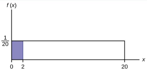
In this case, the area equals the area of a rectangle from [latex]x=0[/latex] to [latex]x=2[/latex]. The area of a rectangle is [latex]\mbox{base} \times \mbox{height}[/latex], so
[latex]\displaystyle{\mbox{Area}=(2-0) \times \frac{1}{20}=0.1}[/latex]
The area corresponds to the probability that the associated continuous random variable takes on a value between [latex]x=0[/latex] and [latex]x=2[/latex]. Because the area is 0.1, the probability that [latex]0 \lt x \lt 2[/latex] is 0.1. Mathematically, we can write this as:
[latex]\displaystyle{P(0 \lt x \lt 2)=0.1}[/latex]
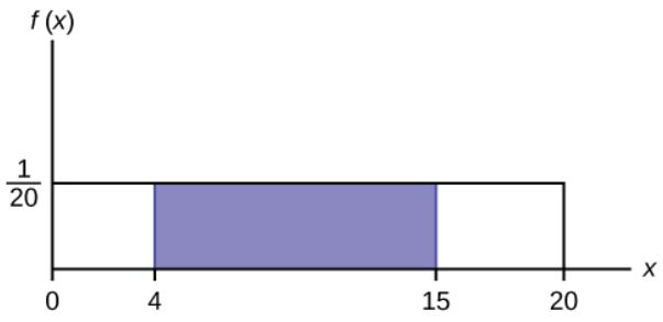
Suppose we want to find the probability that the random variable takes on a value between [latex]x=4[/latex] and [latex]x=15[/latex]. This corresponds to the area under the curve in between [latex]x=4[/latex] and [latex]x=15[/latex].
[latex]\displaystyle{\mbox{Area}=P(4 \lt x \lt 15)=(15-4) \times \frac{1}{20}=0.55}[/latex]
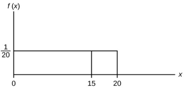
Suppose we want to find [latex]P(x=15)[/latex]. This corresponds to the area above [latex]x=15[/latex], which is just a vertical line. A vertical line has no width (or zero width). So
[latex]\displaystyle{\mbox{Area}=P(x=15)=0 \times \frac{1}{20}=0}[/latex]
NOTE
The probability density function [latex]\displaystyle{f(x)=\frac{1}{20}}[/latex] used above is an example of a uniform distribution. The graph of a uniform distribution is always a horizontal line.
TRY IT
Consider the probability density function [latex]\displaystyle{f(x)=\frac{1}{8}}[/latex] for [latex]0 \leq x \leq 8[/latex]. Draw the graph of [latex]f(x)[/latex] and find [latex]P(2.5 \lt x \lt 7.5)[/latex].
Click to see Solution
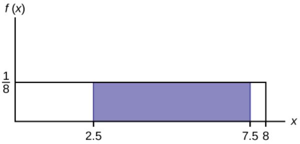
[latex]\displaystyle{P(2.5 \lt x \lt 7.5)=(7.5-2.5) \times \frac{1}{8}=0.625}[/latex]
Watch this video: Continuous probability distribution intro by Khan Academy [9:57]
Concept Review
The probability density function describes the curve of a continuous random variables. The area under the probability density curve between two points corresponds to the probability that the variable falls between those two values. In other words, the area under the probability density curve between points [latex]a[/latex] and [latex]b[/latex] is equal to [latex]P(a \lt x \lt b)[/latex].
If [latex]X[/latex] is a continuous random variable, the probability density function, [latex]f(x)[/latex], is used to draw the graph of the probability distribution. The total area under the graph of [latex]f(x)[/latex] is one. The area under the graph of [latex]f(x)[/latex] and between values [latex]a[/latex] and [latex]b[/latex] gives the probability [latex]P(a \lt x \lt b)[/latex].
Attribution
“5.1 Continuous Probability Functions“ in Introductory Statistics by OpenStax is licensed under a Creative Commons Attribution 4.0 International License.
