8.7 Hypothesis Tests for a Population Mean with Unknown Population Standard Deviation

Valerie Watts

8.7 Hypothesis Tests for a Population Mean with Unknown Population Standard Deviation

LEARNING OBJECTIVES

Conduct and interpret hypothesis tests for a population mean with unknown population standard deviation.

Some notes about conducting a hypothesis test:

The null hypothesis [latex]H_0[/latex] is always an “equal to.” The null hypothesis is the original claim about the population parameter.
The alternative hypothesis [latex]H_a[/latex] is a “less than,” “greater than,” or “not equal to.” The form of the alternative hypothesis depends on the context of the question.
The form of the alternative hypothesis tell us if the test is left-tail, right-tail, or two-tail. The alternative hypothesis is the key to conducting the test and finding the correct p-value.
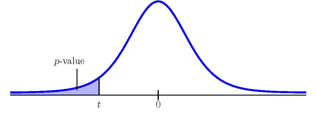
- If the alternative hypothesis is a “less than”, then the test is left-tail. The p-value is the area in the left-tail of the distribution.
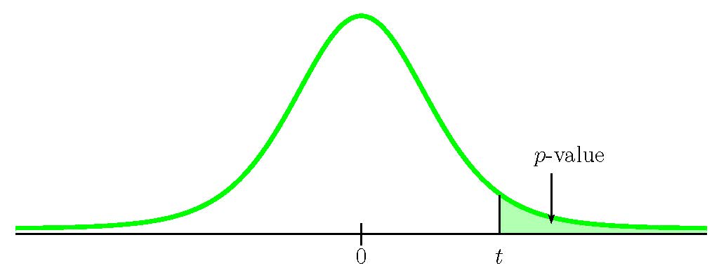
- If the alternative hypothesis is a “greater than”, then the test is right-tail. The p-value is the area in the right-tail of the distribution.
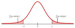
- If the alternative hypothesis is a “not equal to”, then the test is two-tail. The p-value is the sum of the area in the two-tails of the distribution. Each tail represents exactly half of the p-value.
Think about the meaning of the p-value. A data analyst (and anyone else) should have more confidence that they made the correct decision to reject the null hypothesis with a smaller p-value (for example, 0.001 as opposed to 0.04) even if using a significance level of 0.05. Similarly, for a large p-value such as 0.4, as opposed to a p-value of 0.056 (a significance level of 0.05 is less than either number), a data analyst should have more confidence that they made the correct decision in not rejecting the null hypothesis. This makes the data analyst use judgment rather than mindlessly applying rules.
The significance level must be identified before collecting the sample data and conducting the test. Generally, the significance level will be included in the question. If no significance level is given, a common standard is to use a significance level of 5%.
An alternative approach for hypothesis testing is to use what is called the critical value approach. In this book, we will only use the p-value approach. Some of the videos below may mention the critical value approach, but this approach will not be used in this book.

Steps to Conduct a Hypothesis Test for a Population Mean with Unknown Population Standard Deviation

Write down the null and alternative hypotheses in terms of the population mean [latex]\mu[/latex]. Include appropriate units with the values of the mean.
Use the form of the alternative hypothesis to determine if the test is left-tailed, right-tailed, or two-tailed.
Collect the sample information for the test and identify the significance level [latex]\alpha[/latex].
When the population standard deviation is unknown, the p-value is the area in the corresponding tail of the [latex]t[/latex]-distribution with:
[latex]\begin{eqnarray*} t & = & \frac{\overline{x}-\mu}{\frac{s}{\sqrt{n}}} \\ \\ df & = & n-1 \\ \\ \end{eqnarray*}[/latex]
Compare the p-value to the significance level and state the outcome of the test:
- If p-value[latex]\leq \alpha[/latex], reject [latex]H_0[/latex] in favour of [latex]H_a[/latex].
  - The results of the sample data are significant. There is sufficient evidence to conclude that the null hypothesis [latex]H_0[/latex] is an incorrect belief and that the alternative hypothesis [latex]H_a[/latex] is most likely correct.
- If p-value[latex]\gt \alpha[/latex], do not reject [latex]H_0[/latex].
  - The results of the sample data are not significant. There is not sufficient evidence to conclude that the alternative hypothesis [latex]H_a[/latex] may be correct.
Write down a concluding sentence specific to the context of the question.

USING EXCEL TO CALCULE THE P-VALUE FOR A HYPOTHESIS TEST ON A POPULATION MEAN WITH UNKNOWN POPULATION STANDARD DEVIATION

The p-value for a hypothesis test on a population mean is the area in the tail(s) of the distribution of the sample mean. When the population standard deviation is unknown, use the [latex]t[/latex]-distribution to find the p-value.

If the p-value is the area in the left-tail:

Use the t.dist function to find the p-value. In the t.dist(t-score, degrees of freedom, logic operator) function:
- For t-score, enter the value of [latex]t[/latex] calculated from [latex]\displaystyle{t=\frac{\overline{x}-\mu}{\frac{s}{\sqrt{n}}}}[/latex].
- For degrees of freedom, enter the degrees of freedom for the [latex]t[/latex]-distribution [latex]n-1[/latex].
- For the logic operator, enter true. Note: Because we are calculating the area under the curve, we always enter true for the logic operator.
The output from the t.dist function is the area under the [latex]t[/latex]-distribution to the left of the entered [latex]t[/latex]-score.
Visit the Microsoft page for more information about the t.dist function.

If the p-value is the area in the right-tail:

Use the t.dist.rt function to find the p-value. In the t.dist.rt(t-score, degrees of freedom) function:
- For t-score, enter the value of [latex]t[/latex] calculated from [latex]\displaystyle{t=\frac{\overline{x}-\mu}{\frac{s}{\sqrt{n}}}}[/latex].
- For degrees of freedom, enter the degrees of freedom for the [latex]t[/latex]-distribution [latex]n-1[/latex].
The output from the t.dist.rt function is the area under the [latex]t[/latex]-distribution to the right of the entered [latex]t[/latex]-score.
Visit the Microsoft page for more information about the t.dist.rt function.

If the p-value is the sum of area in the tails:

Use the t.dist.2t function to find the p-value. In the t.dist.2t(t-score, degrees of freedom) function:
- For t-score, enter the absolute value of [latex]t[/latex] calculated from [latex]\displaystyle{t=\frac{\overline{x}-\mu}{\frac{s}{\sqrt{n}}}}[/latex]. Note: In the t.dist.2t function, the value of the [latex]t[/latex]-score must be a positive number. If the [latex]t[/latex]-score is negative, enter the absolute value of the [latex]t[/latex]-score into the t.dist.2t function.
- For degrees of freedom, enter the degrees of freedom for the [latex]t[/latex]-distribution [latex]n-1[/latex].
The output from the t.dist.2t function is the sum of areas in the tails under the [latex]t[/latex]-distribution.
Visit the Microsoft page for more information about the t.dist.2t function.

EXAMPLE

Statistics students believe that the mean score on the first statistics test is 65. A statistics instructor thinks the mean score is higher than 65. He samples ten statistics students and obtains the following scores:

65	67	66	68	72
65	70	63	63	71

The instructor performs a hypothesis test using a 1% level of significance. The test scores are assumed to be from a normal distribution.

Solution:

Hypotheses:

[latex]\begin{eqnarray*} H_0: & & \mu=65 \\ H_a: & & \mu \gt 65 \end{eqnarray*}[/latex]

p-value:

From the question, we have [latex]n=10[/latex], [latex]\overline{x}=67[/latex], [latex]s=3.1972...[/latex] and [latex]\alpha=0.01[/latex].

This is a test on a population mean where the population standard deviation is unknown (we only know the sample standard deviation [latex]s=3.1972...[/latex]). So we use a [latex]t[/latex]-distribution to calculate the p-value. Because the alternative hypothesis is a [latex]\gt[/latex], the p-value is the area in the right-tail of the distribution.

This is a t-distribution curve. The peak of the curve is at 0 on the horizontal axis. The point t is also labeled. A vertical line extends from point t to the curve with the area to the right of this vertical line shaded. The p-value equals the area of this shaded region.

To use the t.dist.rt function, we need to calculate out the [latex]t[/latex]-score:

[latex]\begin{eqnarray*} t & = & \frac{\overline{x}-\mu}{\frac{s}{\sqrt{n}}} \\ & = & \frac{67-65}{\frac{3.1972...}{\sqrt{10}}} \\ & = & 1.9781... \end{eqnarray*}[/latex]

The degrees of freedom for the [latex]t[/latex]-distribution is [latex]n-1=10-1=9[/latex].

Function

t.dist.rt

Answer

Field 1

1.9781….

0.0396

Field 2

9

So the p-value[latex]=0.0396[/latex].

Conclusion:

Because p-value[latex]=0.0396 \gt 0.01=\alpha[/latex], we do not reject the null hypothesis. At the 1% significance level there is not enough evidence to suggest that mean score on the test is greater than 65.

NOTES

The null hypothesis [latex]\mu=65[/latex] is the claim that the mean test score is 65.
The alternative hypothesis [latex]\mu \gt 65[/latex] is the claim that the mean test score is greater than 65.
Keep all of the decimals throughout the calculation (i.e. in the sample standard deviation, the [latex]t[/latex]-score, etc.) to avoid any round-off error in the calculation of the p-value. This ensures that we get the most accurate value for the p-value.
The p-value is the area in the right-tail of the [latex]t[/latex]-distribution, to the right of [latex]t=1.9781...[/latex].
The p-value of 0.0396 tells us that under the assumption that the mean test score is 65 (the null hypothesis), there is a 3.96% chance that the mean test score is 65 or more. Compared to the 1% significance level, this is a large probability, and so is likely to happen assuming the null hypothesis is true. This suggests that the assumption that the null hypothesis is true is most likely correct, and so the conclusion of the test is to not reject the null hypothesis.

TRY IT

A company claims that the average change in the value of their stock is $3.50 per week. An investor believes this average is too high. The investor records the changes in the company’s stock price over 30 weeks and finds the average change in the stock price is $2.60 with a standard deviation of $1.80. At the 5% significance level, is the average change in the company’s stock price lower than the company claims?

Click to see Solution

Hypotheses:

[latex]\begin{eqnarray*} H_0: & & \mu=$3.50 \\ H_a: & & \mu \lt $3.50 \end{eqnarray*}[/latex]

p-value:

From the question, we have [latex]n=30[/latex], [latex]\overline{x}=2.6[/latex], [latex]s=1.8[/latex] and [latex]\alpha=0.05[/latex].

This is a test on a population mean where the population standard deviation is unknown (we only know the sample standard deviation [latex]s=1.8.[/latex]). So we use a [latex]t[/latex]-distribution to calculate the p-value. Because the alternative hypothesis is a [latex]\lt[/latex], the p-value is the area in the left-tail of the distribution.

his is a t-distribution curve. The peak of the curve is at 0 on the horizontal axis. The point t is also labeled. A vertical line extends from point t to the curve with the area to the left of this vertical line shaded. The p-value equals the area of this shaded region.

To use the t.dist function, we need to calculate out the [latex]t[/latex]-score:

[latex]\begin{eqnarray*} t & = & \frac{\overline{x}-\mu}{\frac{s}{\sqrt{n}}} \\ & = & \frac{2.6-3.5}{\frac{1.8}{\sqrt{30}}} \\ & = & -1.5699... \end{eqnarray*}[/latex]

The degrees of freedom for the [latex]t[/latex]-distribution is [latex]n-1=30-1=29[/latex].

Function

t.dist

Answer

Field 1

-1.5699….

0.0636

Field 2

29

Field 3

true

So the p-value[latex]=0.0636[/latex].

Conclusion:

Because p-value[latex]=0.0636 \gt 0.05=\alpha[/latex], we do not reject the null hypothesis. At the 5% significance level there is not enough evidence to suggest that average change in the stock price is lower than $3.50.

NOTES

The null hypothesis [latex]\mu=$3.50[/latex] is the claim that the average change in the company’s stock is $3.50 per week.
The alternative hypothesis [latex]\mu \lt $3.50[/latex] is the claim that the average change in the company’s stock is less than $3.50 per week.
The p-value is the area in the left-tail of the [latex]t[/latex]-distribution, to the left of [latex]t=-1.5699...[/latex].
The p-value of 0.0636 tells us that under the assumption that the average change in the stock is $3.50 (the null hypothesis), there is a 6.36% chance that the average change is $3.50 or less. Compared to the 5% significance level, this is a large probability, and so is likely to happen assuming the null hypothesis is true. This suggests that the assumption that the null hypothesis is true is most likely correct, and so the conclusion of the test is to not reject the null hypothesis. In other words, the company’s claim that the average change in their stock price is $3.50 per week is most likely correct.

EXAMPLE

A paint manufacturer has their production line set-up so that the average volume of paint in a can is 3.78 liters. The quality control manager at the plant believes that something has happened with the production and the average volume of paint in the cans has changed. The quality control department takes a sample of 100 cans and finds the average volume is 3.62 liters with a standard deviation of 0.7 liters. At the 5% significance level, has the volume of paint in a can changed?

Solution:

Hypotheses:

[latex]\begin{eqnarray*} H_0: & & \mu=3.78 \mbox{ liters} \\ H_a: & & \mu \neq 3.78 \mbox{ liters} \end{eqnarray*}[/latex]

p-value:

From the question, we have [latex]n=100[/latex], [latex]\overline{x}=3.62[/latex], [latex]s=0.7[/latex] and [latex]\alpha=0.05[/latex].

This is a test on a population mean where the population standard deviation is unknown (we only know the sample standard deviation [latex]s=0.7[/latex]). So we use a [latex]t[/latex]-distribution to calculate the p-value. Because the alternative hypothesis is a [latex]\neq[/latex], the p-value is the sum of area in the tails of the distribution.

To use the t.dist.2t function, we need to calculate out the [latex]t[/latex]-score:

[latex]\begin{eqnarray*} t & = & \frac{\overline{x}-\mu}{\frac{s}{\sqrt{n}}} \\ & = & \frac{3.62-3.78}{\frac{0.07}{\sqrt{100}}} \\ & = & -2.2857... \end{eqnarray*}[/latex]

The degrees of freedom for the [latex]t[/latex]-distribution is [latex]n-1=100-1=99[/latex].

Function

t.dist.2t

Answer

Field 1

2.2857….

0.0244

Field 2

99

So the p-value[latex]=0.0244[/latex].

Conclusion:

Because p-value[latex]=0.0244 \lt 0.05=\alpha[/latex], we reject the null hypothesis in favour of the alternative hypothesis. At the 5% significance level there is enough evidence to suggest that average volume of paint in the cans has changed.

NOTES

The null hypothesis [latex]\mu=3.78[/latex] is the claim that the average volume of paint in the cans is 3.78.
The alternative hypothesis [latex]\mu \neq 3.78[/latex] is the claim that the average volume of paint in the cans is not 3.78.
Keep all of the decimals throughout the calculation (i.e. in the [latex]t[/latex]-score) to avoid any round-off error in the calculation of the p-value. This ensures that we get the most accurate value for the p-value.
The p-value is the sum of the area in the two tails. The output from the t.dist.2t function is exactly the sum of the area in the two tails, and so is the p-value required for the test. No additional calculations are required.
The t.dist.2t function requires that the value entered for the [latex]t[/latex]-score is positive. A negative [latex]t[/latex]-score entered into the t.dist.2t function generates an error in Excel. In this case, the value of the [latex]t[/latex]-score is negative, so we must enter the absolute value of this [latex]t[/latex]-score into field 1.
The p-value of 0.0244 is a small probability compared to the significance level, and so is unlikely to happen assuming the null hypothesis is true. This suggests that the assumption that the null hypothesis is true is most likely incorrect, and so the conclusion of the test is to reject the null hypothesis in favour of the alternative hypothesis. In other words, the average volume of paint in the cans has most likely changed from 3.78 liters.

_{Watch this video: Hypothesis Testing: t-test, right tail by ExcelIsFun [11:02]}

_{Watch this video: Hypothesis Testing: t-test, left tail by ExcelIsFun [7:48]}

_{Watch this video: Hypothesis Testing: t-test, two tail by ExcelIsFun [8:54]}

Concept Review

The hypothesis test for a population mean is a well established process:

Write down the null and alternative hypotheses in terms of the population mean [latex]\mu[/latex]. Include appropriate units with the values of the mean.
Use the form of the alternative hypothesis to determine if the test is left-tailed, right-tailed, or two-tailed.
Collect the sample information for the test and identify the significance level.
When the population standard deviation is unknown, find the p-value (the area in the corresponding tail) for the test using the [latex]t[/latex]-distribution with [latex]\displaystyle{t=\frac{\overline{x}-\mu}{\frac{s}{\sqrt{n}}}}[/latex] and [latex]df=n-1[/latex].
Compare the p-value to the significance level and state the outcome of the test.
Write down a concluding sentence specific to the context of the question.

Attribution

“9.6 Hypothesis Testing of a Single Mean and Single Proportion“ in Introductory Statistics by OpenStax is licensed under a Creative Commons Attribution 4.0 International License.

License

Icon for the Creative Commons Attribution-NonCommercial-ShareAlike 4.0 International License