12.5 The Regression Equation
LEARNING OBJECTIVES
- Find the equation of the line-of-best fit.
- Use the line-of-best-fit to make predictions.
We often want to use values of the independent variable to make predictions about the value of the dependent variable. For example, we might want to use the amount a business spends on advertising each quarter to make a prediction about the revenue the business will generate that quarter. When a linear relationship exists between an independent and dependent variable, we can build a linear model of that relationship, and then we can use that model to make predictions about the dependent variable.
Simple linear regression is a modeling technique in which the linear relationship between one independent variable [latex]x[/latex] and one dependent variable [latex]y[/latex] is approximated by a straight line, called the line-of-best-fit or least squares line. It is important to note that the line-of-best-fit only models the linear relationship between the independent and dependent variables.
The equation for the regression line is:
[latex]\begin{eqnarray*} \hat{y} & = & b_0+b_1x \\ \\ \hat{y} & = & \mbox{predicted value of } y \\ x & = & \mbox{value of the independent variable} \\ b_0 & = &y\mbox{-interecept of the line} \\ b_1 & = & \mbox{slope of the line} \end{eqnarray*}[/latex]
The value of [latex]\hat{y}[/latex] is the estimated value of [latex]y[/latex]. It is the value of [latex]y[/latex] obtained using the regression line. It is not generally equal to the value of [latex]y[/latex] from the sample data. The values for the slope [latex]b_1[/latex] and the [latex]y[/latex]-intercept [latex]b_0[/latex] in the line-of-best-fit are calculated using the sample data and the least squares method. Although there are formulas to calculate the values of the slope and [latex]y[/latex]-intercept in the regression line, we will calculate the slope and [latex]y[/latex]-intercept using the built-in functions in Excel.
The slope of the linear regression equation:
- The slope of the line-of-best-fit [latex]b_1[/latex] and the correlation coefficient [latex]r[/latex] have the same sign. That is, [latex]b_1[/latex] and [latex]r[/latex] are either both positive or both negative.
- The slope [latex]b_1[/latex] of the regression equation tells us how the dependent variable [latex]y[/latex] changes for a one unit increase in the independent variable [latex]x[/latex].
- When interpreting the slope, be specific to the context of the question, using the actual names of the variable and correct units.
The [latex]y[/latex]-intercept of the linear regression equation:
- The [latex]y[/latex]-intercept [latex]b_0[/latex] of the line-of-best-fit is the predicted value of the dependent variable [latex]y[/latex] when [latex]x=0[/latex].
- When interpreting the [latex]y[/latex]-intercept, be specific to the context of the question, using the actual names of the variable and correct units.
CALCULATING THE SLOPE AND [latex]\textcolor{white}y[/latex]-INTERCEPT OF THE LINEAR REGRESSION EQUATION IN EXCEL
To calculate the slope of the linear regression equation, use the slope(array for y’s,array for x’s) function.
- For array for y’s, enter the cell array containing the dependent variable [latex]y[/latex] data.
- For array for x’s, enter the cell array containing the independent variable [latex]x[/latex] data.
Visit the Microsoft page for more information about the slope function.
To calculate the [latex]y[/latex]-intercept of the linear regression equation, use the intercept(array for y’s,array for x’s) function.
- For array for y’s, enter the cell array containing the dependent variable [latex]y[/latex] data.
- For array for x’s, enter the cell array containing the independent variable [latex]x[/latex] data.
Visit the Microsoft page for more information about the intercept function.
NOTE
The order in which the data is entered into these functions is important. In both the slope and intercept functions, the data for the dependent variable is entered in the first array and the data for the independent variable is entered in the second array. The output from the slope and intercept function will be different when the order of the inputs are switched.
EXAMPLE
A statistics professor wants to study the relationship between a student’s score on the third exam in the course and their final exam score. The professor took a random sample of 11 students and recorded their third exam score (out of 80) and their final exam score (out of 200). The results are recorded in the table below. The professor wants to develop a linear regression model to predict a student’s final exam score from the third exam score.
| Student | Third Exam Score | Final Exam Score |
| 1 | 65 | 175 |
| 2 | 67 | 133 |
| 3 | 71 | 185 |
| 4 | 71 | 163 |
| 5 | 66 | 126 |
| 6 | 75 | 198 |
| 7 | 67 | 153 |
| 8 | 70 | 163 |
| 9 | 71 | 159 |
| 10 | 69 | 151 |
| 11 | 69 | 159 |
- Find the equation for the line-of-best-fit.
- Interpret the slope of the line-of-best fit.
Solution:
- Because we want to predict the final exam score from the third exam score, the independent variable [latex]x[/latex] is the third exam score and the dependent variable [latex]y[/latex] is the final exam score. Enter the data into an Excel spreadsheet. For this example, suppose we entered the data (without the column headings) so that the student column is in column A from A1 to A11, the third exam score is in column B from B1 to B11, and the final exam score is in column C from C1 to C11.
Function slope Answer Field 1 C1:C11 4.83 Field 2 B1:B11 Function intercept Answer Field 1 C1:C11 -173.51 Field 2 B1:B11 The equation for the line-of-best-fit is [latex]\hat{y}=-173.51+4.83x[/latex] where [latex]x[/latex] is the third exam score and [latex]\hat{y}[/latex] is the (predicted) final exam score.
The graph below shows the scatter diagram with the line-of-best-fit.

- The slope is [latex]b_1=4.83[/latex]. Interpretation: For a one point increase in the score on the third exam, the final exam score increases by 4.83 points.
NOTE
- When writing down the linear regression equation, remember to define what the variables represent in the context of the question. That is, state what [latex]x[/latex] and [latex]\hat{y}[/latex] represent in relation to the question.
- When writing down the interpretation of the slope, remember to be specific to the question using the actual names of the independent and dependent variables and appropriate units.
Making Predictions with the Linear Regression Equation
Given a specific value of the independent variable [latex]x[/latex], the linear regression equation may be used to predict/estimate the value of the dependent variable [latex]y[/latex]. To make predictions, the following condition must be met:
- There must be a linear relationship between the variables. The stronger the linear relationship, the better the prediction will be.
- The linear regression equation is only valid to predict values of the dependent variable. That is, we may only use the equation to solve for [latex]\hat{y}[/latex] for a given value of [latex]x[/latex], and not the other way around.
- The linear regression equation should only be used to make predictions for [latex]y[/latex] for values of [latex]x[/latex] within the domain of the [latex]x[/latex] values in the sample data used to construct the regression equation. The regression equation does not provide reliable predictions for values of [latex]x[/latex] that fall outside the domain of the [latex]x[/latex] values in the sample data.
EXAMPLE
A statistics professor wants to study the relationship between a student’s score on the third exam in the course and their final exam score. The professor took a random sample of 11 students and recorded their third exam score (out of 80) and their final exam score (out of 200). The results are recorded in the table below. The professor developed the linear regression model [latex]\hat{y}=-173.51+4.83x[/latex] to predict a student’s final exam score ([latex]\hat{y}[/latex]) from a student’s third exam score ([latex]x[/latex]).
| Student | Third Exam Score | Final Exam Score |
| 1 | 65 | 175 |
| 2 | 67 | 133 |
| 3 | 71 | 185 |
| 4 | 71 | 163 |
| 5 | 66 | 126 |
| 6 | 75 | 198 |
| 7 | 67 | 153 |
| 8 | 70 | 163 |
| 9 | 71 | 159 |
| 10 | 69 | 151 |
| 11 | 69 | 159 |
- What is the professor’s final exam prediction for a student that scored 66 on the third exam?
- What is the professor’s final exam prediction for a student that scored 73 on the third exam?
- Should the professor use the linear regression model to predict the final exam score for a student that scored 90 on the third exam? Why?
Solution:
- Substitute [latex]x=66[/latex] into the linear regression equation:
[latex]\begin{eqnarray*}\\ \hat{y} & = & -173.51+4.83*66 \\ & = & 145.27 \end{eqnarray*}[/latex]
A student that scored 66 on the third exam has a predicted score of 145.27 on the final exam.
- Substitute [latex]x=73[/latex] into the linear regression equation:
[latex]\begin{eqnarray*}\\ \hat{y} & = & -173.51+4.83*73 \\ & = & 179.08 \end{eqnarray*}[/latex]
A student that scored 73 on the third exam has a predicted score of 179.08 on the final exam.
- The [latex]x[/latex] values (third exam score) in the sample data are between 65 and 75. An [latex]x[/latex] value of 90 is outside the domain of the observed [latex]x[/latex] values in the data. So, we cannot reliably predict the final exam score for a student that scored 90 on the third exam. Of course, it is possible to enter [latex]x=90[/latex] into the linear regression equation and calculate the corresponding value of [latex]\hat{y}[/latex], but this value is not a reliable prediction. If we calculate out the value of [latex]\hat{y}[/latex] in the regression equation for [latex]x=90[/latex], we get [latex]\hat{y}=261.19[/latex], a value that makes no sense in the context of the question because the maximum score on the final exam is 200.
NOTES
- The values obtained for the linear regression equation are predictions only. Here, 145.27 is the predicted final exam score for a student that scored 66 on the third exam. This does not mean that a student that actually scored 66 on the third exam will score 145.27 on the final exam.
- Remember that the linear regression only gives reliable predictions for values of [latex]x[/latex] that fall within the domain of [latex]x[/latex] values in the sample data.
TRY IT
SCUBA divers have maximum dive times they cannot exceed when going to different depths. The data in the table below shows different depths with the maximum dive times in minutes.
| Depth (in feet) | Maximum Dive Time (in minutes) |
| 50 | 80 |
| 60 | 55 |
| 70 | 45 |
| 80 | 35 |
| 90 | 25 |
| 100 | 22 |
- Find the linear regression equation to predict the maximum dive time from the depth.
- Interpret the slope of the regression equation found in part 1.
- Predict the maximum dive time for a depth of 75 feet.
Click to see Solution
- [latex]\displaystyle{\hat{y}=127.24-1.11x}[/latex] where [latex]x[/latex] is the depth in feet and [latex]\hat{y}[/latex] is the (predicted) maximum dive time in minutes.
- For each one foot increase in depth, the maximum dive time decreases by 1.11 minutes.
- [latex]\displaystyle{\hat{y}=127.24-1.11*75=43.99 \mbox{ minutes}}[/latex]
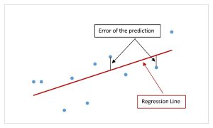
Errors and The Least Squares Method
The difference between the actual value of the dependent variable [latex]y[/latex] (in the sample date) and the predicted value of the dependent variable [latex]\hat{y}[/latex] obtained from the linear regression equation is called the error or residual.
[latex]\begin{eqnarray*} \mbox{Error} & = & \mbox{Actual Value}-\mbox{Predicted Value} \\ & = & y-\hat{y}\end{eqnarray*}[/latex]
Graphically, the absolute value of the error is the vertical distance between the actual value of [latex]y[/latex] (the point on the scatter diagram) and the predicted value of [latex]\hat{y}[/latex] (the point on the linear regression line). In other words, the absolute value of the error measures the vertical distance between the actual data point and the line.
The slope and [latex]y[/latex]-intercept for the linear regression equation are generated using the errors and the least squares method. The idea behind finding the line-of-best-fit is based on the assumption that the data are scattered about a straight line. For any line, the errors can be calculated, squared, and then these squared errors can be added up. Of all of the possible lines, the line-of-best-fit is the one line that minimizes this sum of the squared errors. Any other line will have a higher sum of the squared errors compared to the sum of the squared errors for the line-of-best-fit.
Watch this video: Slope and Intercept for Linear Regression in Excel by ExcelIsFun [18:29]
Concept Review
A regression line, or a line-of best-fit, can be drawn on a scatter diagram and used to predict outcomes for the [latex]y[/latex] variable in a given data set or sample data. Regression lines can be used to predict values within the given set of data, but should not be used to make predictions for values outside the set of data.
Attribution
“12.3 The Regression Equation“ and “12.5 Prediction“ in Introductory Statistics by OpenStax is licensed under a Creative Commons Attribution 4.0 International License.
