7.5 Calculating the Sample Size for a Confidence Interval
LEARNING OBJECTIVES
- Calculate the minimum sample size required to estimate a population parameter.
Usually we have no control over the sample size of a data set. However, if we are able to set the sample size, as in cases where we are taking a survey, it is very helpful to know just how large it should be to provide the most information. Sampling can be very costly, in both time and product. Simple telephone surveys will cost approximately $30.00 each, for example, and some sampling requires the destruction of the product. Selecting a sample that is too large is expensive and time consuming. But selecting a sample that is too small can lead to inaccurate conclusions. We want to find the minimum sample size required to achieve the desired level of accuracy in the confidence interval.
Calculating the Sample Size for a Population Mean
The margin of error [latex]E[/latex] for a confidence interval for a population mean is
[latex]\displaystyle{E=\frac{z \times \sigma}{\sqrt{n}}}[/latex]
where [latex]z[/latex] is the [latex]z[/latex]-score so that the area under the standard normal distribution in between [latex]-z[/latex] and [latex]z[/latex] is the confidence level [latex]C[/latex].
Rearranging this formula for [latex]n[/latex] we get a formula for the sample size [latex]n[/latex]:
[latex]\displaystyle{n=\left(\frac{z \times \sigma}{E}\right)^2}[/latex]
In order to use this formula, we need values for [latex]z[/latex], [latex]E[/latex] and [latex]\sigma[/latex]:
- The value for [latex]z[/latex] is determined by the confidence level of the interval, calculated the same way we calculate the [latex]z[/latex]-score for a confidence interval.
- The value for the margin of error [latex]E[/latex] is set as the predetermined acceptable error, or tolerance, for the difference between the sample mean [latex]\overline{x}[/latex] and the population mean [latex]\mu[/latex]. In other words, [latex]E[/latex] is set to the maximum allowable width of the confidence interval.
- An estimate for the population standard deviation [latex]\sigma[/latex] can be found by one of the following methods:
- Conduct a small pilot study and use the sample standard deviation from the pilot study.
- Use the sample standard deviation from previously collected data. Although crude, this method of estimating the standard deviation may help reduce costs significantly.
- Use [latex]\displaystyle{\frac{\mbox{Range}}{4}}[/latex] where [latex]\mbox{Range}[/latex] is the difference between the maximum and minimum values of the population under study.
NOTES
- Although we do not know the population standard deviation when calculating the sample size, we do not use the [latex]t[/latex]-distribution in the sample size formula. In order to use the [latex]t[/latex]-distribution in this situation, we need the degrees of freedom [latex]n-1[/latex]. But [latex]n[/latex] is the sample size we are trying to estimate. So, we must use the normal distribution to determine the sample size.
- The value of [latex]n[/latex] determined from the formula is the minimum sample size required to achieve the desired level of confidence. The sample size [latex]n[/latex] is a count, and so is an integer. It would be unusual for the value of [latex]n[/latex] generated by the formula to be an integer. Because [latex]n[/latex] is the minimum sample size required, we must round the output from the formula up to the next integer. If we round the value of [latex]n[/latex] down, the sample size will be below the minimum required sample size.
- After we have found the sample size [latex]n[/latex] and collected the data for the sample, we use the appropriate confidence interval formula and the sample standard deviation from the actual sample (assuming [latex]\sigma[/latex] is unknown), and not the estimate of the standard deviation used in the calculation of the sample size.
CALCULATING THE [latex]\textcolor{white}z[/latex]-SCORE FOR SAMPLE SIZE IN EXCEL
To find the [latex]z[/latex]-score to calculate the sample size for a confidence interval with confidence level [latex]C[/latex], use the norm.s.inv(area to the left of z) function.
- For area to the left of z, enter the entire area to the left of the [latex]z[/latex]-score you are trying to find. For a confidence interval, the area to the left of [latex]z[/latex] is [latex]\displaystyle{C+\frac{1-C}{2}}[/latex].
The output from the norm.s.inv function is the value of [latex]z[/latex]-score needed to find the sample size.
EXAMPLE
We want to estimate the mean age of Foothill College students. From previous information, an estimate of the standard deviation of the ages of the students is 15 years. We want to be 95% confident that the sample mean age is within two years of the population mean age. How many randomly selected Foothill College students must be surveyed to achieved the desired level of accuracy?
Solution:
To find the sample size, we need to find the [latex]z[/latex]-score for the 95% confidence interval. This means that we need to find the [latex]z[/latex]-score so that the entire area to the left of [latex]z[/latex] is [latex]\displaystyle{0.95+\frac{1-0.95}{2}=0.975}[/latex].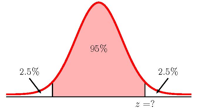
| Function | norm.s.inv | Answer |
| Field 1 | 0.975 | 1.9599… |
So [latex]z=1.9599....[/latex]. From the question [latex]\sigma \simeq 15[/latex] and [latex]E=2[/latex].
[latex]\begin{eqnarray*}\\ n & = & \left(\frac{z \times \sigma}{E}\right)^2 \\ & = & \left( \frac{1.9599... \times 15}{2}\right)^2 \\ & = & 216.08... \\ & \Rightarrow & 217 \mbox{ students} \\ \\ \end{eqnarray*}[/latex]
217 students must be surveyed to achieve the desired accuracy.
NOTE
Remember to round the value for the sample size UP to the next integer. This ensures that the sample size is an integer and is large enough. Do not forget to include appropriate units with the sample size.
TRY IT
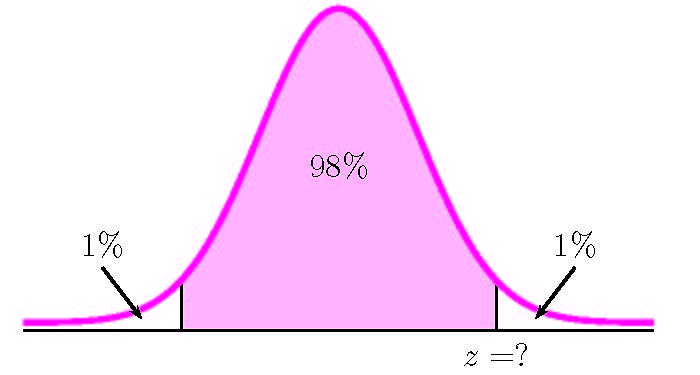
You want to estimate the height of all high school basketball players. You want to be 98% confident with a margin of error of 1.5. From a small pilot study, you estimate the standard deviation to be 3 inches. How large a sample do you need to take to achieve the desired level of accuracy?
Click to see Solution
| Function | norm.s.inv | Answer |
| Field 1 | 0.99 | 2.3263… |
 [latex]\begin{eqnarray*} n & = & \left(\frac{z \times \sigma}{E}\right)^2 \\ & = & \left(\frac{2.3263... \times 3}{1.5}\right)^2 \\ & = & 21.6487... \\& \Rightarrow & 22 \mbox{ high school basketball players}\end{eqnarray*}[/latex]
Calculating the Sample Size for a Population Proportion
The margin of error [latex]E[/latex] for a confidence interval for a population proportion is
[latex]\displaystyle{E=z \times \sqrt{\frac{p \times (1-p)}{n}}}[/latex]
where [latex]z[/latex] is the [latex]z[/latex]-score so that the area under the standard normal distribution in between [latex]-z[/latex] and [latex]z[/latex] is the confidence level [latex]C[/latex].
Rearranging this formula for [latex]n[/latex] we get a formula for the sample size [latex]n[/latex]:
[latex]\displaystyle{n=p \times (1-p) \times \left(\frac{z}{E}\right)^2}[/latex]
In order to use this formula, we need values for [latex]z[/latex], [latex]E[/latex] and [latex]p[/latex]:
- The value for [latex]z[/latex] is determined by the confidence level of the interval, calculated the same way we calculate the [latex]z[/latex]-score for a confidence interval.
- The value for the margin of error [latex]E[/latex] is set as the predetermined acceptable error, or tolerance, for the difference between the sample proportion [latex]\hat{p}[/latex] and the population proportion [latex]p[/latex]. In other words, [latex]E[/latex] is set to the maximum allowable width of the confidence interval.
- An estimate for the population proportion [latex]p[/latex]. If no estimate for the population proportion is provided, we use [latex]p=0.5[/latex].
NOTES
- The value of [latex]n[/latex] determined from the formula is the minimum sample size required to achieve the desired level of confidence. The sample size [latex]n[/latex] is a count, and so is an integer. It would be unusual for the value of [latex]n[/latex] generated by the formula to be an integer. Because [latex]n[/latex] is the minimum sample size required, we must round the output from the formula up to the next integer. If we round the value of [latex]n[/latex] down, the sample size will be below the minimum required sample size.
- After we have found the sample size [latex]n[/latex] and collected the data for the sample, we use the appropriate confidence interval formula and the sample proportion from the actual sample.
- By using [latex]0.5[/latex] as an estimate for [latex]p[/latex] in the sample size formula we will get the largest required sample size for the confidence level and margin of error we selected. This is true because of all combinations of two fractions (the values of [latex]p[/latex] and [latex]1-p[/latex]) that add to one, the largest multiple is when each is 0.5. Without any other information concerning the population parameter [latex]p[/latex], this is the common practice. This may result in oversampling, but certainly not under sampling.
There is an interesting trade-off between the level of confidence and the sample size that shows up here when considering the cost of sampling. The table below shows the appropriate sample size at different levels of confidence and different margins of error, assuming [latex]p=0.5[/latex]. Looking at each row, we can see that for the same margin of error, a higher level of confidence requires a larger sample size. Similarly, looking at each column, we can see that for the same confidence level, a smaller margin of error requires a larger sample size.
| Required Sample Size (90%) | Required Sample Size (95%) | Margin of Error |
| 1691 | 2401 | 2% |
| 752 | 1067 | 3% |
| 271 | 384 | 5% |
| 68 | 96 | 10% |
EXAMPLE
Suppose a mobile phone company wants to determine the current percentage of customers aged 50+ who use text messaging on their cell phones. How many customers aged 50+ should the company survey in order to be 90% confident with a margin of error of 3%?.
Solution:
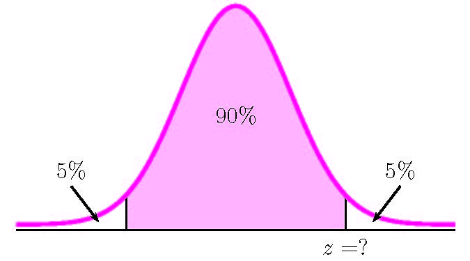
To find the sample size, we need to find the [latex]z[/latex]-score for the 90% confidence interval. This means that we need to find the [latex]z[/latex]-score so that the entire area to the left of [latex]z[/latex] is [latex]\displaystyle{0.90+\frac{1-0.90}{2}=0.95}[/latex].
| Function | norm.s.inv | Answer |
| Field 1 | 0.95 | 1.6448… |
So [latex]z=1.6.448....[/latex]. From the question [latex]E=0.03[/latex]. Because no estimate of the population proportion is given, [latex]p=0.5[/latex].
[latex]\begin{eqnarray*} \\ n & = & p \times (1-p) \times \left(\frac{z }{E}\right)^2 \\ & = & 0.5 \times (1-0.5) \times \left( \frac{1.6448...}{0.03}\right)^2 \\ & = & 751.539... \\ & \Rightarrow & 752 \mbox{ customers age 50+} \\ \\ \end{eqnarray*}[/latex]
752 customers aged 50+ must be surveyed to achieve the desired accuracy.
NOTE
Remember to round the value for the sample size UP to the next integer. This ensures that the sample size is large enough. Do not forget to include appropriate units with the sample size.
TRY IT
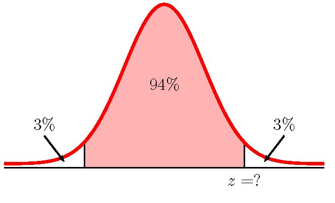
Suppose an internet marketing company wants to determine the percentage of customers who click on ads on their smartphones. How many customers should the company survey in order to be 94% confident that the estimated proportion is within 5% of the population proportion of customers who click on ads on their smartphones?
Click to see Solution
| Function | norm.s.inv | Answer |
| Field 1 | 0.97 | 1.8807… |
 [latex]\begin{eqnarray*} n & = & p \times (1-p) \times \left(\frac{z}{E}\right)^2 \\ & = & 0.5 \times (1-0.5) \times \left(\frac{1.8807...}{0.05}\right)^2 \\ & = & 353.738... \\& \Rightarrow & 354 \mbox{ customers}\end{eqnarray*}[/latex]
Watch this video: Sample Size for Confidence Intervals by ExcelIsFun [7:54]
Concept Review
In order to construct a confidence interval, a sample is taken from the population under study. But collecting sample information is time consuming and expensive. The minimum sample size required to achieve the desired level of accuracy is determined before collecting the sample data.
- Sample size for population means: [latex]\displaystyle{n=\left(\frac{z \times \sigma}{E}\right)^2}[/latex]
- Sample size for population proportions: [latex]\displaystyle{n=p \times (1-p) \times \left(\frac{z}{E}\right)^2}[/latex]
After calculating the value of [latex]n[/latex] from the formula, round the value of [latex]n[/latex] up to the next integer.
Attribution
“7.2 The Central Limit Theorem for Sums“ in Introductory Statistics by OpenStax is licensed under a Creative Commons Attribution 4.0 International License.
“8.4 Calculating the Sample Size n: Continuous and Binary Random Variables“ in Introductory Business Statistics by OpenStax is licensed under a Creative Commons Attribution 4.0 International License.
