5.1 Introduction to Continuous Random Variables

A continuous random variable corresponds to data that can be measured. Continuous random variables have many applications. Baseball batting averages, IQ scores, the length of time a long distance telephone call lasts, the amount of money a person carries, the length of time a computer chip lasts, and SAT scores are just a few examples of continuous random variables. The field of reliability depends on a variety of continuous random variables.
NOTE
The values of discrete and continuous random variables can be ambiguous. For example, if [latex]X[/latex] is equal to the number of miles (to the nearest mile) you drive to work, then [latex]X[/latex] is a discrete random variable because you count the miles. If [latex]X[/latex] is the distance you drive to work, then [latex]X[/latex] is a continuous random variable because you measure the miles. For a second example, if [latex]X[/latex] is equal to the number of books in a backpack, then [latex]X[/latex] is a discrete random variable because the number of books is a count. If [latex]X[/latex] is the weight of a book, then [latex]X[/latex] is a continuous random variable because weights are measured. How the random variable is defined is very important.
Properties of Continuous Probability Distributions
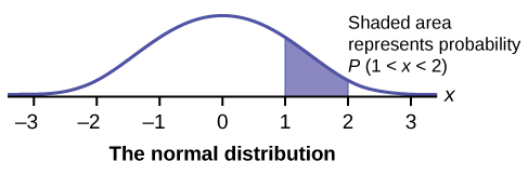
The graph of a continuous probability distribution is a curve. The probability a continuous random variable takes on a value in an interval is the area under the curve of the distribution of the continuous random variable. Properties of of a continuous random variable [latex]X[/latex] include:
- The outcomes are measured, not counted.
- The entire area under the curve of the distribution of the continuous random variable and above the [latex]x[/latex]-axis is equal to one.
- Probability is found for intervals of [latex]x[/latex] values rather than for individual [latex]x[/latex] values.
- [latex]P(c \lt x \lt d)[/latex] is the probability that the random variable [latex]X[/latex] is in the interval between the values of [latex]c[/latex] and [latex]d[/latex]. The value of [latex]P(c \lt x \lt d)[/latex] is the area under the curve, above the [latex]x[/latex]-axis, to the right of [latex]c[/latex] and the left of [latex]d[/latex].
- The probability that [latex]x[/latex] takes on any single individual value is zero—that is, [latex]P(x=c)=0[/latex]. The area below the curve, above the [latex]x[/latex]-axis, and between [latex]x=c[/latex] and [latex]x=c[/latex] has no width, and therefore no area. Because the probability is equal to the area and the area is 0, the probability is also 0.
- Because probability is equal to area and [latex]P(x=c)=0[/latex], [latex]P(c \lt x \lt d)[/latex] is the same as [latex]P(c \leq x \leq d)[/latex].
Generally, calculate is needed to find the area under the curve of many continuous probability distributions. However, we will use the built-in functions in Excel to calculate the area under the continuous probability distribution functions. There are many different continuous probability distributions, including the uniform distribution and the exponential distribution. We will focus on the most important continuous probability distribution—the normal distribution.
Attribution
“Chapter 5 Introduction” in Introductory Statistics by OpenStax is licensed under a Creative Commons Attribution 4.0 International License.
