5.3 The Normal Distribution
LEARNING OBJECTIVES
- Describe properties of the normal distribution.
- Apply the Empirical Rule for normal distributions.
The normal distribution is the most important of all the distributions. It is widely used and even more widely abused. Its graph is a symmetric, bell-shaped curve. You see the bell curve in almost all disciplines, including psychology, business, economics, the sciences, nursing, and, of course, mathematics. Some of your instructors may use the normal distribution to help determine your grade. Most IQ scores are normally distributed. Often real-estate prices fit a normal distribution. The normal distribution is extremely important, but it cannot be applied to everything in the real world.
Properties of the normal distribution include:
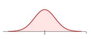
- The curve of a normal distribution is symmetric and bell-shaped.
- The center of a normal distribution is at the mean [latex]\mu[/latex].
- In a normal distribution, the mean, the median, and the mode are equal.
- The curve is symmetric about a vertical line drawn through the mean.
- The tails of a normal distribution extend to infinity in both directions along the [latex]x[/latex]-axis.
- The standard deviation, [latex]\sigma[/latex], of a normal distribution determines how wide or narrow the curve is.
- The total area under the curve of a normal distribution equals 1.
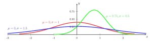
A normal distribution is completely determined by its mean [latex]\mu[/latex] and its standard deviation [latex]\sigma[/latex], which means there are an infinite number of normal distributions. The mean [latex]\mu[/latex] determines the center of the distribution—a change in the value of [latex]\mu[/latex] causes the graph to shift to the left or right. The standard deviation [latex]\sigma[/latex] determines the shape of the bell. Because the area under the curve must equal one, a change in the standard deviation [latex]\sigma[/latex] causes a change in the shape of the curve—the curve becomes fatter or skinnier depending on the value of [latex]\sigma[/latex].
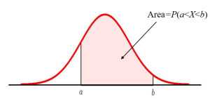
The normal distribution is a continuous probability distribution. As we saw in the previous section, the area under the curve of the normal distribution equals the probability that the corresponding normal random variable takes on a value with in a given interval. That is, the probability that the normal random variable is in between [latex]a[/latex] and [latex]b[/latex] equals the area under the normal curve in between [latex]x=a[/latex] and [latex]x=b[/latex].
Watch this video: ck12.org normal distribution problems: Quantitative sense of normal distributions | Khan Academy by Khan Academy [10:52]
The Empirical Rule
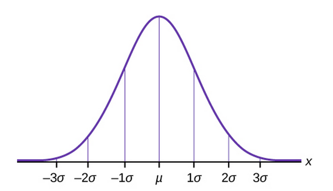
For a normal distribution with mean [latex]\mu[/latex] and standard deviation [latex]\sigma[/latex], then the Empirical Rule says the following:
- About [latex]68\%[/latex] of the values lie between [latex]–1 \times \sigma[/latex] and [latex]+1 \times \sigma[/latex] of the mean [latex]\mu[/latex].
- In other words, about [latex]68\%[/latex] of the data fall with one standard deviation of the mean.
- About [latex]95\%[/latex] of the values lie between [latex]–2 \times \sigma[/latex] and [latex]+2 \times \sigma[/latex] of the mean [latex]\mu[/latex].
- In other words, about [latex]95\%[/latex] of the data fall with two standard deviation of the mean.
- About [latex]99.7\%[/latex] of the values lie between [latex]–3 \times \sigma[/latex] and [latex]+3 \times \sigma[/latex] of the mean [latex]\mu[/latex].
- In other words, about [latex]99.7\%[/latex] of the data fall with three standard deviation of the mean
The empirical rule is also known as the [latex]68-95-99.7[/latex] rule.
EXAMPLE
Suppose a normal distribution has a mean [latex]50[/latex] and a standard deviation [latex]6[/latex].
About [latex]68\%[/latex] of the values lie between [latex]–1 \times \sigma = -1 \times 6 = –6[/latex] and [latex]1 \times \sigma = 1 \times 6 = 6[/latex] of the mean [latex]50[/latex]. The values [latex]50 – 6 = 44[/latex] and [latex]50 + 6 = 56[/latex] are within one standard deviation of the mean [latex]50[/latex]. So [latex]68\%[/latex] of the values in this distribution are between 44 and 56.
About [latex]95\%[/latex] of the values lie between [latex]–2 \times \sigma = -2 \times 6 = –12[/latex] and [latex]2 \times \sigma = 2 \times 6 = 12[/latex] of the mean [latex]50[/latex]. The values [latex]50 – 12 = 38[/latex] and [latex]50 + 12 = 62[/latex] are within two standard deviations of the mean [latex]50[/latex]. So [latex]95\%[/latex] of the values in the distribution are between 38 and 62.
About [latex]99.7\%[/latex] of the [latex]x[/latex] values lie between [latex]–3 \times \sigma = -3 \times 6 = –18[/latex] and [latex]3 \times \sigma = 3 \times 6 = 18[/latex] of the mean [latex]50[/latex]. The values [latex]50 – 18 = 32[/latex] and [latex]50 + 18= 68[/latex] are within three standard deviations of the mean [latex]50[/latex]. So [latex]99.7\%[/latex] of the values in the distribution are between 32 and 68.
TRY IT
Suppose a normal distribution has a mean [latex]25[/latex] and a standard deviation [latex]5[/latex]. Between what values of does [latex]68\%[/latex] of the data lie?
Click to see Solution
- Between [latex]25+(-1) \times 5=20[/latex] and [latex]25+1 \times 5=30[/latex].
EXAMPLE
From 1984 to 1985, the height of 15 to 18-year-old males from Chile follows a normal distribution with mean [latex]172.36[/latex]cm and standard deviation [latex]6.34[/latex]cm.
- About [latex]68\%[/latex] of the heights of 15 to 18-year old males in Chile from 1984 to 1985 lie between what two values?
- About [latex]95\%[/latex] of the heights of 15 to 18-year old males in Chile from 1984 to 1985 lie between what two values?
- About [latex]99.7\%[/latex] of the heights of 15 to 18-year old males in Chile from 1984 to 1985 lie between what two values?
Solution:
- [latex]\displaystyle{\mu+(-1)\times \sigma=172.36+(-1)\times 6.34=166.02}[/latex] and [latex]\displaystyle{\mu+1 \times \sigma=172.36+1 \times 6.34=178.70}[/latex]
- [latex]\displaystyle{\mu+(-2)\times \sigma=172.36+(-2)\times 6.34=159.68}[/latex] and [latex]\displaystyle{\mu+2 \times \sigma=172.36+2 \times 6.34=185.04}[/latex]
- [latex]\displaystyle{\mu+(-3)\times \sigma=172.36+(-1)\times 6.34=153.34}[/latex] and [latex]\displaystyle{\mu+3 \times \sigma=172.36+2 \times 6.34=191.36}[/latex]
TRY IT
The scores on a college entrance exam have an approximate normal distribution with a mean [latex]52[/latex] points and a standard deviation of [latex]11[/latex] points.
- About [latex]68\%[/latex] of the exam scores lie between what two values?
- About [latex]95\%[/latex] of the exam scores lie between what two values?
- About [latex]99.7\%[/latex] of the exam scores lie between what two values?
Click to see Solution
- About [latex]68\%[/latex] of the scores lie between the values [latex]52+(-1) \times 11=41[/latex] and [latex]52+1 \times 11=63[/latex].
- About [latex]95\%[/latex] of the values lie between the values [latex]52+(-2) \times 11=30[/latex] and [latex]52+2 \times 11=74[/latex].
- About [latex]99.7\%[/latex] of the values lie between the values [latex]52+(-3) \times 11=19[/latex] and [latex]52+3 \times 11=85[/latex].
Watch this video: Empirical Rule| Probability and Statistics | Khan Academy by Khan Academy [10:25]
Concept Review
The normal distribution is the most frequently used distribution in statistics. The graph of a normal distribution is a symmetric, bell-shaped curve centered at the mean of the distribution. The probability that a normal random variable takes on a value in inside an interval equals the area under the corresponding normal distribution curve.
For a normal distribution, the empirical rule states that 68% of the data falls within one standard deviation of the mean, 95% of the data falls within two standard deviations, and 99.7% of the data falls within three standard deviations of the mean.
Attribution
“6.1 The Standard Normal Distribution” in Introductory Statistics by OpenStax is licensed under a Creative Commons Attribution 4.0 International License.
