7.4 Confidence Intervals for a Population Proportion
LEARNING OBJECTIVES
- Calculate and interpret confidence intervals for estimating a population proportion.
During an election year, we see articles in the newspaper that state confidence intervals in terms of proportions or percentages. For example, a poll for a particular candidate running for president might show that the candidate has 40% of the vote within three percentage points (if the sample is large enough). Often, election polls are calculated with 95% confidence, so, the pollsters would be 95% confident that the true proportion of voters who favored the candidate would be between 37% and 43%.
Investors in the stock market are interested in the true proportion of stocks that go up and down each week. Businesses that sell personal computers are interested in the proportion of households in the United States that own personal computers. Confidence intervals can be calculated for the true proportion of stocks that go up or down each week and for the true proportion of households in the United States that own personal computers.
A confidence interval for a population proportion is based on the fact that the sample proportions follow an approximately normal distribution when both [latex]n \times p \geq 5[/latex] and [latex]n \times (1-p) \geq 5[/latex]. Similar to confidence intervals for population means, a confidence interval for a population proportion is constructed by taking a sample of size [latex]n[/latex] from the population, calculating the sample proportion [latex]\hat{p}[/latex], and then adding and subtracting the margin of error from [latex]\hat{p}[/latex] to get the limits of the confidence interval.
In order to construct a confidence interval for a population proportion, we must be able to assume the sample proportions follow a normal distribution. As we have seen previously, we can assume the sample proportions follow a normal distribution when both [latex]n \times p \geq 5[/latex] and [latex]n \times (1-p) \geq 5[/latex]. But in this situation, the population proportion [latex]p[/latex] is unknown so we cannot check the values of [latex]n \times p[/latex] and [latex]n \times (1-p)[/latex]. Because we must take a sample and calculate the sample proportion [latex]\hat{p}[/latex], we can check the quantities [latex]n \times \hat{p}[/latex] and [latex]n \times (1-\hat{p})[/latex]. For the confidence interval, if both [latex]n \times \hat{p} \geq 5[/latex] and [latex]n \times (1-\hat{p}) \geq 5[/latex], we can assume the sample proportions follow a normal distribution.
Calculating the Margin of Error
The margin of error for a confidence interval with confidence level [latex]C[/latex] for an unknown population proportion [latex]p[/latex] is
[latex]\displaystyle{\mbox{Margin of Error}=z \times \sqrt{\frac{\hat{p} \times (1-\hat{p})}{n}}}[/latex]
where [latex]z[/latex] is the the [latex]z[/latex]-score so the area the left of [latex]z[/latex] is [latex]\displaystyle{C+\frac{1-C}{2}}[/latex].
NOTE
In the margin of error formula, the sample proportion [latex]\hat{p}[/latex] is used to estimate the unknown population proportion [latex]p[/latex]. The estimated sample proportion [latex]\hat{p}[/latex] is used because [latex]p[/latex] is the unknown quantity we are trying to estimate with the confidence interval. The sample proportion [latex]\hat{p}[/latex] is calculated from the sample taken to construct the confidence interval where
[latex]\displaystyle{\hat{p}=\frac{\mbox{number of items in the sample with characteristic of interest}}{n}}[/latex]
Constructing the Confidence Interval
The limits for the confidence interval with confidence level [latex]C[/latex] for an unknown population proportion [latex]p[/latex] are
[latex]\begin{eqnarray*} \\ \mbox{Lower Limit} & = & \hat{p}-z \times \sqrt{\frac{\hat{p} \times (1-\hat{p})}{n}} \\ \\ \mbox{Upper Limit} & = & \hat{p}+z \times \sqrt{\frac{\hat{p} \times (1-\hat{p})}{n}} \\ \\ \end{eqnarray*}[/latex]
where [latex]z[/latex] is the [latex]z[/latex]-score so the area to the left of [latex]z[/latex] is [latex]\displaystyle{C+\frac{1-C}{2}}[/latex].
NOTE
The confidence interval can only be used if we can assume the sample proportions follow a normal distribution. This means we must check that [latex]n \times \hat{p} \geq 5[/latex] and [latex]n \times (1-\hat{p}) \geq 5[/latex] before constructing the confidence interval. If one of [latex]n \times \hat{p}[/latex] or [latex]n \times (1-\hat{p})[/latex] is less than 5, we cannot construct the confidence interval.
CALCULATING THE [latex]{\color{white}z}[/latex]-SCORE FOR A CONFIDENCE INTERVAL IN EXCEL
To find the [latex]z[/latex]-score to construct a confidence interval with confidence level [latex]C[/latex], use the norm.s.inv(area to the left of z) function.
- For area to the left of z, enter the entire area to the left of the [latex]z[/latex]-score you are trying to find. For a confidence interval, the area to the left of [latex]z[/latex] is [latex]\displaystyle{C+\frac{1-C}{2}}[/latex].
The output from the norm.s.inv function is the value of [latex]z[/latex]-score needed to construct the confidence interval.
NOTE
The norm.s.inv function requires that we enter the entire area to the left of the unknown [latex]z[/latex]-score. This area includes the confidence level (the area in the middle of the distribution) plus the remaining area in the left tail.
EXAMPLE
Suppose that a market research firm is hired to estimate the percent of adults living in a large city who have cell phones. Five hundred randomly selected adult residents in this city are surveyed to determine whether they have cell phones. Of the 500 people surveyed, 421 responded yes – they own cell phones.
- Construct a 95% confidence interval for the proportion of adult residents of this city who have cell phones.
- Interpret the confidence interval found in part 1.
- Is it reasonable to conclude that 85% of the adult residents of this city have cell phones? Explain.
Solution:
- The sample proportion is [latex]\displaystyle{\hat{p}=\frac{421}{500}=0.842}[/latex]. We need to check [latex]n \times \hat{p}[/latex] and [latex]n \times (1-\hat{p})[/latex]:
[latex]\begin{eqnarray*} \\ n \times \hat{p} & = & 500 \times 0.842=421 \geq 5 \\ \\ n \times (1-\hat{p}) & = & 500 \times (1-0.842)=79\geq 5 \\ \\ \end{eqnarray*}[/latex]
Because both [latex]n \times \hat{p} \geq 5[/latex] and [latex]n \times (1-\hat{p}) \geq 5[/latex], the sample proportions follow a normal distribution and we can construct the confidence interval.
To find the confidence interval, we need to find the [latex]z[/latex]-score for the 95% confidence interval. This means that we need to find the [latex]z[/latex]-score so that the entire area to the left of [latex]z[/latex] is [latex]\displaystyle{0.95+\frac{1-0.95}{2}=0.975}[/latex].
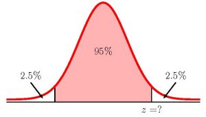
Function norm.s.inv Answer Field 1 0.975 1.9599… So [latex]z=1.9599....[/latex]. The 95% confidence interval is
[latex]\begin{eqnarray*}\\\mbox{Lower Limit}&=&\hat{p}-z\times\sqrt{\frac{\hat{p}\times(1-\hat{p})}{n}}\\&=&0.842-1.9599...\times\sqrt{\frac{0.842\times(1-0.842)}{500}}\\&=&0.8100\\\\ \mbox{Upper Limit}&=&\hat{p}+z\times\sqrt{\frac{\hat{p}\times(1-\hat{p})}{n}}\\&=&0.842+1.9599...\times\sqrt{\frac{0.842\times(1-0.842)}{500}}\\&=&0.8740\\\\\end{eqnarray*}[/latex]
- We are 95% confident that the proportion of adult residents of this city who have cell phones is between 81% and 87.4%.
- It is reasonable to conclude that 85% of the adult residents of this city have cell phones because 85% is inside the confidence interval.
NOTES
- When calculating the limits for the confidence interval keep all of the decimals in the [latex]z[/latex]-score and other values throughout the calculation. This will ensure that there is no round-off error in the answers. You can use Excel to do the calculation of the limits, clicking on the cells containing the [latex]z[/latex]-score and any other values, to ensure that all of the decimal places are used in the calculation.
- The limits for the confidence interval are percents. For example, the upper limit of 0.8740 is the decimal form of a percent: 87.4%.
- When writing down the interpretation of the confidence interval, make sure to include the confidence level, the actual population proportion captured by the confidence interval (i.e. be specific to the context of the question), and express the limits as percents.
- 95% of all confidence interval constructed this way contain the proportion of adult residents in this city that have a cell phone. For example, if we constructed 100 of these confidence (using 100 different samples of size 500), we would expect 95 of them to contain the true proportion of adult residents in this city that have a cell phone.
TRY IT
Suppose 250 randomly selected people are surveyed to determine if they own a tablet. Of the 250 surveyed, 98 reported owning a tablet.
- Construct a 94% confidence interval for the proportion of people who own tablets.
- Interpret the confidence interval found in part 1.
- Is it reasonable to assume that 30% of people own tablets? Explain.
Click to see Solution
-
Function norm.s.inv Answer Field 1 0.97 1.8807… 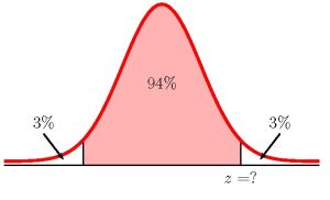 [latex]\begin{eqnarray*}\\\mbox{Lower Limit}&=&\hat{p}-z\times\sqrt{\frac{\hat{p}\times(1-\hat{p})}{n}}\\&=&0.392-1.8807...\times\sqrt{\frac{0.392\times(1-0.392)}{250}}\\&=&0.3339\\\\\mbox{Upper Limit}&=&\hat{p}+z\times\sqrt{\frac{\hat{p}\times(1-\hat{p})}{n}}\\&=&0.392+1.8807...\times\sqrt{\frac{0.392\times(1-0.392)}{250}}\\&=&0.4501\\\\\end{eqnarray*}[/latex]
 - We are 94% confident that the proportion of people who own tablets is between 33.39% and 45.01%.
- It is not reasonable to claim the proportion of people who own tablets is 30% because 30% is outside the confidence interval.
EXAMPLE
For a class project, a political science student at a large university wants to estimate the percent of students who are registered voters. He surveys 500 students and finds that 300 are registered voters.
- Construct a 90% confidence interval for the percent of students who are registered voters.
- Interpret the confidence interval found in part 1.
Solution:
- The sample proportion is [latex]\displaystyle{\hat{p}=\frac{300}{500}=0.6}[/latex]. We need to check [latex]n \times \hat{p}[/latex] and [latex]n \times (1-\hat{p})[/latex]:
[latex]\begin{eqnarray*}\\n\times\hat{p}&=&500\times0.6=300\geq 5\\\\ n\times(1-\hat{p})&=&500\times(1-0.6)=200\geq 5\\\\\end{eqnarray*}[/latex]
Because both [latex]n \times \hat{p} \geq 5[/latex] and [latex]n \times (1-\hat{p}) \geq 5[/latex], the sample proportions follow a normal distribution and we can construct the confidence interval.
To find the confidence interval, we need to find the [latex]z[/latex]-score for the 90% confidence interval. This means that we need to find the [latex]z[/latex]-score so that the entire area to the left of [latex]z[/latex] is [latex]\displaystyle{0.90+\frac{1-0.90}{2}=0.95}[/latex].
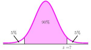
Function norm.s.inv Answer Field 1 0.95 1.6448… So [latex]z=1.6448....[/latex]. The 90% confidence interval is
[latex]\begin{eqnarray*}\\\mbox{Lower Limit}&=&\hat{p}-z\times\sqrt{\frac{\hat{p}\times(1-\hat{p})}{n}}\\&=&0.6-1.6448...\times \sqrt{\frac{0.6\times(1-0.6)}{500}}\\&=&0.5640\\\\\mbox{Upper Limit}&=&\hat{p}+z\times\sqrt{\frac{\hat{p}\times(1-\hat{p})}{n}}\\&=&0.6+1.6448...\times\sqrt{\frac{0.6\times(1-0.6)}{500}}\\&=&0.6360\\\\\end{eqnarray*}[/latex]
- We are 90% confident that the percent of students who are registered voters is between 56.4% and 63.6%.
TRY IT
A student polls her school to see if students in the school district are for or against the new legislation regarding school uniforms. She surveys 600 students and finds that 480 are against the new legislation.
- Construct a 98% confidence interval for the proportion of students who are against the new legislation.
- Interpret the confidence interval found in part 1.
- A parents group claims that only 75% of students are against the legislation. Is it reasonable for the group to make this claim? Explain.
Click to see Solution
-
Function norm.s.inv Answer Field 1 0.99 2.3263… 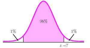 [latex]\begin{eqnarray*}\\\mbox{Lower Limit}&=&\hat{p}-z\times\sqrt{\frac{\hat{p}\times(1-\hat{p})}{n}}\\&=&0.8-2.3264...\times\sqrt{\frac{0.8 \times(1-0.8)}{600}}\\&=&0.7620\\\\\mbox{Upper Limit}&=&\hat{p}+z\times\sqrt{\frac{\hat{p}\times(1-\hat{p})}{n}}\\&=&0.8 +2.3263...\times\sqrt{\frac{0.8\times(1-0.8)}{600}}\\&=&0.8380\\\\\end{eqnarray*}[/latex]
 - We are 98% confident that the proportion of students who are against the new legislation is between 76.20% and 83.80%.
- It is not reasonable for the group to claim the proportion is 75% because 75% is outside of the confidence interval.
Watch this video: Confidence Interval for a population proportion by Excel is Fun [8:34]
Watch this video: Confidence Interval for a population proportion by Excel is Fun [4:51]
Concept Review
Some statistical measures, like many survey questions, measure qualitative rather than quantitative data. In this case, the population parameter being estimated is a proportion. It is possible to create a confidence interval for the true population proportion following procedures similar to those used in creating confidence intervals for population means. The formulas are slightly different, but they follow the same reasoning.
The general form for a confidence interval for a single population proportion is given by
[latex]\begin{eqnarray*}\\\mbox{Lower Limit}&=&\hat{p}-\times\sqrt{\frac{\hat{p}\times(1-\hat{p})}{n}}\\\\\mbox{Upper Limit}&=&\hat{p}+z\times\sqrt{\frac{\hat{p}\times(1-\hat{p})}{n}}\\\\\end{eqnarray*}[/latex]
where [latex]z[/latex] is the the [latex]z[/latex]-score so the area to the left of [latex]z[/latex] is [latex]\displaystyle{C+\frac{1-C}{2}}[/latex].
Attribution
“8.3 A Population Proportion“ in Introductory Statistics by OpenStax is licensed under a Creative Commons Attribution 4.0 International License.
