8.5 Rare Events, the Sample, Decision, and Conclusion
LEARNING OBJECTIVES
- Define a rare event and identify how a rare event is used in a hypothesis test.
- Define p-value and significance level and identify how they are used in determining the outcome of a hypothesis test.
Establishing the type of distribution, sample size, and known or unknown population standard deviation can help us figure out how to go about a hypothesis test. However, there are several other factors we should consider when working out a hypothesis test.
Rare Events
Suppose we make an assumption about the value of a population parameter (this assumption is the null hypothesis). We conduct the hypothesis under the assumption that the null hypothesis is true. Then we randomly select a sample from the population. If the sample has properties that would be very unlikely to occur under the assumption the null hypothesis is true, then we would conclude that our assumption about the population is probably incorrect. Remember that our assumption is just an assumption—it is not a fact, and it may or may not be true. But the sample data we collect is real and the information from that sample is a fact that may or may not support the assumption we make about the null hypothesis.
For example, Didi and Ali are at the birthday party of a very wealthy friend. They hurry to be first in line to grab a prize from a tall basket that they cannot see inside of because they will be blindfolded. There are 200 plastic bubbles in the basket and Didi and Ali have been told that there is only one with a $100 bill. Didi is the first person to reach into the basket and pull out a bubble. Her bubble contains a $100 bill. The probability of this happening is [latex]\displaystyle{\frac{1}{200}=0.005}[/latex]. Because this is such an unlikely occurrence, Ali is hoping that what the two of them were told is wrong and there are more $100 bills in the basket. In this case a “rare event” has occurred (Didi getting the $100 bill) so Ali doubts the original assumption about only one $100 bill being in the basket.
A rare event is something we consider to be unlikely to happen (i.e. the probability of that event happening is very small). This is what we are looking for in a hypothesis test. We want to determine if the sample collected for the test is a rare event (unlikely to happen) under the assumption the null hypothesis is true. To determine if the sample is a rare event, we calculate the probability of the sample occurring, assuming that the null hypothesis is true. If the probability of the sample occurring is small, then the sample is a “rare event” and unlikely to occur under the assumption the null hypothesis is true. In such a case we would conclude that the original assumption that the null hypothesis is true must be incorrect, and so we would reject the null hypothesis. If the probability of the sample occurring is not small, then the sample is not a “rare event” and is actually likely to occur under the assumption the null hypothesis is true. In this case we would conclude the original assumption that the null hypothesis is true must be correct, and so we would not reject the null hypothesis.
Remember, a rare event is an event that is unlikely to happen. But unlikely does not mean impossible. The probability of a rare event is very small, which means that the chance of it happening is very small. But as long as the probability is not zero, there is still a possibility the event could happen.
Using the Sample to Test the Null Hypothesis
We use the sample data to calculate the actual probability of getting the selected sample, called the p-value, under the assumption the null hypothesis is true. The p-value is the probability that, if the null hypothesis is true, the results from another randomly selected sample will be as extreme or more extreme as the results obtained from the given sample.
A large p-value calculated from the sample data indicates that we should not reject the null hypothesis. The smaller the p-value, the more unlikely the outcome, and the stronger the evidence is against the null hypothesis. We would reject the null hypothesis if the evidence is strongly against it.
EXAMPLE
The customers of a local bakery claim that the height of the bakery’s bread is, on average, 15 cm. The baker believes his customers are wrong, and that the average height of the bread is more than 15 cm. To persuade his customers that he is right, the baker decides to do a hypothesis test. He bakes 10 loaves of bread. The mean height of the sample loaves is 17 cm. The baker knows from baking hundreds of loaves of bread that the standard deviation for the height is 1 cm and the distribution of the heights is normal. Based on this sample, who is right: the customers or the baker?
Solution:
Here, the population under study is the height of the loaves of bread and [latex]\mu[/latex] is the average height of the loaves of bread.
The customers’ claim is the null hypothesis: [latex]\mu=15[/latex]. The alternative hypothesis is the baker’s claim: [latex]\mu \gt 15[/latex]. In mathematical notation, the hypothesis are
[latex]\begin{eqnarray*} H_0: & & \mu=15 \mbox{ cm} \\ H_a: & & \mu \gt 15 \mbox{ cm} \end{eqnarray*}[/latex]
Because the population standard deviation is known ([latex]\sigma=1[/latex]), the distribution we would use is the normal distribution.
Suppose the null hypothesis is true. That is, suppose [latex]\mu=15[/latex]. Under this assumption, we have to ask if the sample mean of 17 is likely or unlikely to occur. The hypothesis test works by asking the question how unlikely is this sample mean if the null hypothesis is true. The graph shows how far out the sample mean is on the normal curve. The p-value is the probability that, if we took another sample of size 10, any other sample mean would fall at least as far out as 17 cm.
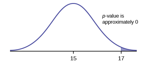
The p-value is the probability that a sample mean is the same or greater than 17 cm when the population mean is, in fact, 15 cm. We can calculate this probability using the normal distribution for sample means. In fact, we are calculating the probability that in a sample of size 10 the sample mean is greater than 17. We learned how to calculate this type of probability when we learned about the sampling distribution of the sample mean:
| Function | 1-norm.dist | Answer |
| Field 1 | 17 | 0.0000000001 |
| Field 2 | 15 | |
| Field 3 | 1/sqrt(10) | |
| Field 4 | true |
So p-value=0.0000000001, which tells us the probability of selecting a sample of size 10 and getting a sample mean greater than 17 is 0.0000000001 under the assumption that the null hypothesis is true ([latex]\mu=15[/latex]). This is a very, very small probability, which tells us that a sample mean of 17 is unlikely to happen if the population mean is 15 cm. Because the sample mean of 17 is so unlikely (meaning it is not happening by chance alone), we conclude that the assumption that the mean is 15 cm is wrong. That is, the evidence provided by the sample is strongly against the claim of the null hypothesis. So we reject the null hypothesis in favour of the alternative hypothesis. That is, based on the test, we believe the null hypothesis is false and the alternative hypothesis is true. So there is enough evidence to suggest that the average height of the loaves of bread is greater than 15 cm.
TRY IT
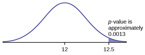
A normal distribution has a standard deviation of 1. The original claim is that the mean of the distribution is 12. An alternative claim is that the mean is greater than 12. The hypotheses are:
[latex]\begin{eqnarray*} H_0: & & \mu=12 \\ H_a: & & \mu \gt 12 \end{eqnarray*}[/latex]
In a sample of 36, the sample mean is 12.5. Calculate the p-value.
Click to see Solution
| Function | 1-norm.dist | Answer |
| Field 1 | 12.5 | 0.0013 |
| Field 2 | 12 | |
| Field 3 | 1/sqrt(36) | |
| Field 4 | true |
p-value=0.0013
Decision and Conclusion
A systematic way to make a decision of whether to reject or not reject the null hypothesis is to compare the p-value and a preset or preconceived value called the significance level, denoted by [latex]\alpha[/latex]. The significance level is the cut-off value for likely versus unlikely when compared to the p-value. When the p-value is greater than the significance level, the sample is likely to occur under the assumption the null hypothesis is true, and so we would fail to reject the null hypothesis. When the p-value is less than or equal to the significance level, the sample is unlikely to occur under the assumption the null hypothesis is true, and so we would reject the null hypothesis in favour of the alternative hypothesis. A preset value for [latex]\alpha[/latex] is the probability of a Type I error (rejecting the null hypothesis when the null hypothesis is true). The significance level may or may not be given at the beginning of the problem.
When we make a decision to reject or not reject H0, do as follows:
- If p-value[latex]\leq \alpha[/latex], reject [latex]H_0[/latex] in favour of [latex]H_a[/latex].
- The results of the sample data are significant. There is sufficient evidence to conclude that the null hypothesis [latex]H_0[/latex] is an incorrect belief and that the alternative hypothesis [latex]H_a[/latex] is most likely correct.
- If p-value[latex]\gt \alpha[/latex], do not reject [latex]H_0[/latex].
- The results of the sample data are not significant. There is not sufficient evidence to conclude that the alternative hypothesis [latex]H_a[/latex] may be correct.
After comparing the p-value and significance level, write a thoughtful conclusion about the hypotheses in terms of the given problem.
TRY IT
A genetics lab claims its product can increase the likelihood a pregnancy will result in a boy being born. Statisticians want to test this claim. Suppose the hypotheses are
[latex]\begin{eqnarray*} H_0: & & p=50\% \\ H_a: & & p \gt 50\% \end{eqnarray*}[/latex]
After conducting the hypothesis test, p-value=0.025. If the significance level is 1%, what is the conclusion of the test?
Click to see Solution
Because the p-value is greater than the significance level (p-value[latex]=0.025 \gt 0.01=\alpha[/latex]), we do not reject the null hypothesis. There is not enough evidence to support the lab’s stated claim that their procedures improve the chances of a boy being born.
Concept Review
A rare event is an event that is unlikely to occur. The probability of a rare event happening is very small. In a hypothesis test, we want to determine if the collected sample is a rare event. The p-value is the probability of getting the sample.
In a hypothesis test, the significance level is the cut-off value for likely versus unlikely. The significance level is compared to the p-value for the test.
- If p-value[latex]\leq \alpha[/latex], reject [latex]H_0[/latex] in favour of [latex]H_a[/latex].
- If p-value[latex]\gt \alpha[/latex], do not reject [latex]H_0[/latex].
After determining the outcome of test, we write a conclusion based on the specific context of the question.
Attribution
“9.4 Rare Events, the Sample, Decision and Conclusion“ in Introductory Statistics by OpenStax is licensed under a Creative Commons Attribution 4.0 International License.
