11.3 Statistical Inference for Two Population Variances
LEARNING OBJECTIVES
- Construct and interpret a confidence interval for two population variances.
- Conduct and interpret a hypothesis test for two population variances.
Sometimes we want to compare the variability between two populations instead of comparing the means of the populations. For example, college administrators would like two college professors grading exams to have the same variation in their grading or a supermarket might be interested in the variability of the check-out times for two checkers.
As with comparing other population parameters, we can construct confidence intervals and conduct hypothesis tests to study the relationship between two population variances. However, because of the distribution we need to use, we study the ratio of two population variances, not the difference in the variances.
Throughout this section, we will use subscripts to identify the values for the sample sizes, variances, and standard deviations for the two populations:
| Symbol for: | Population 1 | Population 2 |
| Population Variance | [latex]\sigma^2_1[/latex] | [latex]\sigma^2_2[/latex] |
| Population Standard Deviation | [latex]\sigma_1[/latex] | [latex]\sigma_2[/latex] |
| Sample Size | [latex]n_1[/latex] | [latex]n_2[/latex] |
| Sample Variance | [latex]s^2_1[/latex] | [latex]s^2_2[/latex] |
| Sample Standard Deviation | [latex]s_1[/latex] | [latex]s_2[/latex] |
In order to construct a confidence interval or conduct a hypothesis test on the ratio of two population variances, [latex]\displaystyle{\frac{\sigma_1^2}{\sigma^2_2}}[/latex], we need to use the distribution of [latex]\displaystyle{\frac{s_1^2}{s^2_2}}[/latex] when the population variances are equal ([latex]\sigma^2_1=\sigma^2_2[/latex]). Suppose we have two normal populations with equal variances [latex]\sigma^2_1=\sigma^2_2[/latex]. A sample of size [latex]n_1[/latex] with sample variance [latex]s^2_1[/latex] is taken from population 1 and a sample of size [latex]n_2[/latex] with sample variance [latex]s^2_2[/latex] is taken from population 2. The sampling distribution of the ratio of the sample variances [latex]\displaystyle{\frac{s_1^2}{s_2^2}}[/latex] follows an [latex]F[/latex]-distribution with [latex]df_1=n_1-1[/latex] and [latex]df_2=n_2-1[/latex].
Constructing a Confidence Interval for the Ratio of Two Population Variances
Suppose a sample of size [latex]n_1[/latex] with sample variance [latex]s^2_1[/latex] is taken from population 1 and a sample of size [latex]n_2[/latex] with sample variance [latex]s^2_2[/latex] is taken from population 2, where the populations are independent and normally distributed. The limits for the confidence interval with confidence level [latex]C[/latex] for the ratio of the population variances [latex]\displaystyle{\frac{\sigma_1^2}{\sigma_2^2}}[/latex] are
[latex]\begin{eqnarray*} \\ \mbox{Lower Limit} & = & \frac{1}{F_R} \times \frac{s_1^2}{s^2_2} \\ \\ \mbox{Upper Limit} & = & \frac{1}{F_L} \times \frac{s_1^2}{s^2_2} \\ \\ \end{eqnarray*}[/latex]
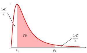
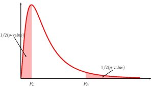
where [latex]F_L[/latex] is the [latex]F[/latex]-score so that the area in the left-tail of the [latex]F[/latex]-distribution is [latex]\displaystyle{\frac{1-C}{2}}[/latex], [latex]F_R[/latex] is the [latex]F[/latex]-score so that the area in the right tail of the [latex]F[/latex]-distribution is [latex]\displaystyle{\frac{1-C}{2}}[/latex] and the [latex]F[/latex]-distribution has degrees of freedom [latex]df_1=n_1-1[/latex] and [latex]df_2=n_2-1[/latex].
NOTES
- Like the other confidence intervals we have seen, the [latex]F[/latex]-scores are the values that trap [latex]C\%[/latex] of the observations in the middle of the distribution so that the area of each tail is [latex]\displaystyle{\frac{1-C}{2}}[/latex].
- Because the [latex]F[/latex]-distribution is not symmetrical, the confidence interval for the ratio of the population variances requires that we calculate two different [latex]F[/latex]-scores: one for the left tail and one for the right tail. In Excel, we will need to use both the f.inv function (for the left tail) and the f.inv.rt function (for the right tail) to find the two different [latex]F[/latex]-scores.
- The [latex]F[/latex]-score for the left tail is part of the formula for the upper limit and the [latex]F[/latex]-score for the right tail is part of the formula for the lower limit. This is not a mistake. It follows from the formula used to determine the limits for the confidence interval.
- It is important that the populations are independent and normally distributed. If the populations are not normal, the confidence interval will not give an accurate result.
EXAMPLE
Two local walk-in medical clinics want to determine if there is any variability in the time patients wait to see a doctor at each clinic. In a sample of 30 patients at Clinic 1, the standard deviation for the wait time to see a doctor was 45 minutes. In a sample of 40 patients at Clinic 2, the standard deviation for the wait time to see a doctor was 27 minutes. Assume the population of wait times at the two clinics are independent and normally distributed.
- Construct a 95% confidence interval for the ratio of the variances for the wait times at the two clinics.
- Interpret the confidence interval found in part 1.
- Is there evidence to suggest that there is a difference in the variances of the wait times at the two clinics? Explain.
Solution:
- Let Clinic 1 be population 1 and Clinic 2 be population 2. From the question we have the following information:
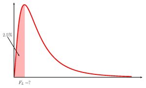
Clinic 1 Clinic 2 [latex]n_1=30[/latex] [latex]n_2=40[/latex] [latex]s_1^2=45^2=2025[/latex] [latex]s^2_2=27^2=729[/latex] To find the confidence interval, we need to find the [latex]F_L[/latex]-score for the 95% confidence interval. This means that we need to find the [latex]F_L[/latex]-score so that the area in the left tail is [latex]\displaystyle{\frac{1-0.95}{2}=0.025}[/latex]. The degrees of freedom for the [latex]F[/latex]-distribution are [latex]df_1=n_1-1=30-1=29[/latex] and [latex]df_2=n_2-1=40-1=39[/latex].
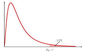
Function f.inv Answer Field 1 0.025 0.4919… Field 2 29 Field 3 39 We also need find the [latex]F_R[/latex]-score for the 95% confidence interval. This means that we need to find the [latex]F_R[/latex]-score so that the area in the right tail is [latex]\displaystyle{\frac{1-0.95}{2}=0.025}[/latex]. The degrees of freedom for the [latex]F[/latex]-distribution are [latex]df_1=n_1-1=30-1=29[/latex] and [latex]df_2=n_2-1=40-1=39[/latex].
Function f.inv.rt Answer Field 1 0.025 1.9618… Field 2 29 Field 3 39 So [latex]F_L=0.4919...[/latex] and [latex]F_R=1.9618...[/latex]. The 95% confidence interval is
[latex]\begin{eqnarray*} \\ \mbox{Lower Limit} & = &\frac{1}{F_R} \times \frac{s_1^2}{s^2_2} \\ & = & \frac{1}{1.9618...} \times \frac{2025}{729} \\ & = & 1.416 \\ \\ \mbox{Upper Limit} & = & \frac{1}{F_L} \times \frac{s_1^2}{s^2_2} \\ & = & \frac{1}{0.4919...} \times \frac{2025}{729} \\ & = & 5.646 \\ \\ \end{eqnarray*}[/latex]
- We are 95% confident that the ratio of the variances in the wait times at the two clinics is between 1.416 and 5.646.
- Because 1 is outside the confidence interval, it suggests that the ratio of the variances [latex]\displaystyle{\frac{\sigma^2_1}{\sigma^2_2}}[/latex] is not 1. If the ratio of the variances cannot equal 1, then the variances cannot be equal. So there is a difference in the variances of the wait times at the two clinics.
NOTES
- When calculating the limits for the confidence interval keep all of the decimals in the [latex]F[/latex]-scores and other values throughout the calculation. This will ensure that there is no round-off error in the answer. You can use Excel to do the calculations of the limits, clicking on the cells containing the [latex]F[/latex]-scores and any other values.
- When writing down the interpretation of the confidence interval, make sure to include the confidence level and the actual ratio of population variances captured by the confidence interval (i.e. be specific to the context of the question). In this case, there are no units for the limits because variance does not have any limits.
Steps to Conduct a Hypothesis Test for Two Population Variances
- Write down the null hypothesis that there is no difference in the population variances:
[latex]\begin{eqnarray*} \\ H_0: & & \sigma^2_1=\sigma^2_2 \end{eqnarray*}[/latex]
The null hypothesis is always the claim that the two population variances are equal.
- Write down the alternative hypotheses in terms of the difference in the population variances. The alternative hypothesis will be one of the following:
[latex]\begin{eqnarray*} \\ H_a: & & \sigma^2_1 \lt \sigma_2^2 \\ H_a: & & \sigma^2_1 \gt \sigma^2_2 \\ H_a: & & \sigma^2_1 \neq \sigma^2_2 \\ \\ \end{eqnarray*}[/latex]
- Use the form of the alternative hypothesis to determine if the test is left-tailed, right-tailed, or two-tailed.
- Collect the sample information for the test and identify the significance level [latex]\alpha[/latex].
- Use the [latex]F[/latex]-distribution to find the p-value (the area in the corresponding tail) for the test. The [latex]F[/latex]-score and degrees of freedom are
[latex]\begin{eqnarray*}F & = & \frac{s_1^2}{s_2^2} \\ \\ df_1 & = & n_1-1 \\ \\ df_2 & = & n_2-1 \\ \\ \end{eqnarray*}[/latex]
- Compare the p-value to the significance level and state the outcome of the test:
- If p-value[latex]\leq \alpha[/latex], reject [latex]H_0[/latex] in favour of [latex]H_a[/latex].
- The results of the sample data are significant. There is sufficient evidence to conclude that the null hypothesis [latex]H_0[/latex] is an incorrect belief and that the alternative hypothesis [latex]H_a[/latex] is most likely correct.
- If p-value[latex]\gt \alpha[/latex], do not reject [latex]H_0[/latex].
- The results of the sample data are not significant. There is not sufficient evidence to conclude that the alternative hypothesis [latex]H_a[/latex] may be correct.
- If p-value[latex]\leq \alpha[/latex], reject [latex]H_0[/latex] in favour of [latex]H_a[/latex].
- Write down a concluding sentence specific to the context of the question.
EXAMPLE
Two college instructors are interested in whether or not there is any variation in the way they grade math exams. They each grade the same set of 30 exams. The first instructor’s grades have a variance of 52.3. The second instructor’s grades have a variance of 89.9. At the 5% significance level, test the claim that the first instructor’s variance is smaller.
Solution:
Let the first instructor’s grades be population 1 and the second instructor’s grades be population 2. From the question we have the following information:
| Instructor 1 | Instructor 2 |
| [latex]n_1=30[/latex] | [latex]n_2=30[/latex] |
| [latex]s_1^2=52.3[/latex] | [latex]s_2^2=89.9[/latex] |
Hypotheses:
[latex]\begin{eqnarray*} H_0: & & \sigma_1^2=\sigma^2_2 \\ H_a: & & \sigma_1^2 \lt \sigma^2_2 \end{eqnarray*}[/latex]
p-value:
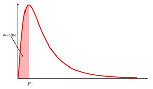
Because the alternative hypothesis is a [latex]\lt[/latex], the p-value is the area in the left tail of the [latex]F[/latex]-distribution.
To use the f.dist function, we need to calculate out the [latex]F[/latex]-score and the degrees of freedom:
[latex]\begin{eqnarray*} F & = &\frac{s_1^2}{s_2^2} \\ & = & \frac{52.3}{89.9} \\ & = & 0.58175... \\ \\ df_1 & = & n_1-1 \\ & = & 30-1 \\ & = & 29 \\ \\df_2 & = & n_2-1 \\ & = & 30-1 \\ & = & 29\end{eqnarray*}[/latex]
| Function | f.dist | Answer |
| Field 1 | 0.58175… | 0.0753 |
| Field 2 | 29 | |
| Field 3 | 29 | |
| Field 4 | true |
So the p-value[latex]=0.0753[/latex].
Conclusion:
Because p-value[latex]=0.0753 \gt 0.05=\alpha[/latex], we do not reject the null hypothesis. At the 5% significance level there is not enough evidence to suggest that the first instructor’s variance is smaller.
NOTES
- The null hypothesis [latex]\sigma_1^2=\sigma^2_2[/latex] is the claim that the variances for the two instructors are equal.
- The alternative hypothesis [latex]\sigma_1^2 \lt \sigma^2_2[/latex] is the claim that the variance for the first instructor’s grades is less than the variance for the second instructor’s grades.
- The p-value is the area in the left tail of the [latex]F[/latex]-distribution, to the left of [latex]F=0.5817...[/latex]. In the calculation of the p-value:
- The function is f.dist because we are finding the area in the left tail of an [latex]F[/latex]-distribution.
- Field 1 is the value of [latex]F[/latex].
- Field 2 is the value of [latex]df_1[/latex].
- Field 3 is the value of [latex]df_2[/latex].
- Field 4 is true.
- The p-value of 0.0753 is a large probability compared to the significance level, and so is likely to happen assuming the null hypothesis is true. This suggests that the assumption that the null hypothesis is true is most likely correct, and so the conclusion of the test is to not reject the null hypothesis. In other words, the variances for the two instructors are most likely equal.
EXAMPLE
A local choral society divides the male singers into tenors and basses. The choral society director wants to know if the variance in the heights of the two groups of singers is the same or different. The director takes a sample from each group and records their height in inches. In a sample of 22 tenors, the sample variance is 3.89. In a sample of 27 basses, the sample variance is 2.72. At the 5% significance level, is there a difference in the heights of the two groups of singers?
Solution:
Let the tenors be population 1 and the basses be population 2. From the question we have the following information:
| Tenors | Basses |
| [latex]n_1=22[/latex] | [latex]n_2=27[/latex] |
| [latex]s_1^2=3.89[/latex] | [latex]s^2=2.72[/latex] |
Hypotheses:
[latex]\begin{eqnarray*} H_0: & & \sigma^2_1=\sigma^2_2 \\ H_a: & & \sigma^2_1 \neq \sigma^2_2 \end{eqnarray*}[/latex]
p-value:
Because the alternative hypothesis is [latex]\neq[/latex], the p-value is the sum of the areas in the tails of the [latex]F[/latex]-distribution.
We need to calculate out the [latex]F[/latex]-score and the degrees of freedom:
[latex]\begin{eqnarray*} F & = &\frac{s_1^2}{s_2^2} \\ & = & \frac{3.89}{2.72} \\ & = & 1.430... \\ \\ df_1 & = & n_1-1 \\ & = & 22-1 \\ & = & 21 \\ \\ df_2 & = & n_2-1 \\ & = & 27-1 \\ & = & 26 \end{eqnarray*}[/latex]
Because this is a two-tailed test, we need to know which tail (left or right) we have the [latex]F[/latex]-score for so that we can use the correct Excel function. If [latex]F \gt 1[/latex], the [latex]F[/latex]-score corresponds to the right tail. If the [latex]F \lt 1[/latex], the [latex]F[/latex]-score corresponds to the left tail. In this case [latex]F=1.430... \gt 1[/latex], so the [latex]F[/latex]-score corresponds to the right tail. We need to use f.dist.rt to find the area in the right tail.
| Function | f.dist.rt | Answer |
| Field 1 | 1.430…. | 0.1919 |
| Field 2 | 21 | |
| Field 3 | 26 |
So the area in the right tail is 0.1919, which means that [latex]\frac{1}{2}[/latex](p-value)=0.1919. This is also the area in the left tail, so
p-value=[latex]0.1919+0.1919=0.3838[/latex]
Conclusion:
Because p-value[latex]=0.3838 \gt 0.05=\alpha[/latex], we do not reject the null hypothesis. At the 5% significance level there is not enough evidence to suggest that there is a difference in the variation in the heights of the two groups of singers.
NOTES
- The null hypothesis [latex]\sigma_1^2=\sigma^2_2[/latex] is the claim that the variances of the heights for the two groups of singers are equal.
- The alternative hypothesis [latex]\sigma_1^2 \neq \sigma^2_2[/latex] is the claim that the variances of the heights for the two groups of singers are not equal
- In a two-tailed hypothesis test for two population variance, we will only have sample information relating to one of the two tails. We must determine which of the tails the sample information belongs to, and then calculate out the area in that tail. The area in each tail represents exactly half of the p-value, so the p-value is the sum of the areas in the two tails.
- If [latex]F \lt 1[/latex], the sample information belongs to the left tail.
- We use f.dist to find the area in the left tail. The area in the right tail equals the area in the left tail, so we can find the p-value by adding the output from this function to itself.
- If [latex]F \gt 1[/latex], the sample information belongs to the right tail.
- We use f.dist.rt to find the area in the right tail. The area in the left tail equals the area in the right tail, so we can find the p-value by adding the output from this function to itself.
- If [latex]F \lt 1[/latex], the sample information belongs to the left tail.
- The p-value of 0.3838 is a large probability compared to the significance level, and so is likely to happen assuming the null hypothesis is true. This suggests that the assumption that the null hypothesis is true is most likely correct, and so the conclusion of the test is to not reject the null hypothesis In other words, the variances in the heights of the two groups of singers are the same.
NOTES
- When two populations have equal variances, the values of [latex]s_1^2[/latex] and [latex]s^2_2[/latex] are close in value. So, the value of [latex]\displaystyle{\frac{s^2_1}{s^2_2}}[/latex] is close to 1. This will result in a large p-value in the hypothesis test and the evidence favours the null hypothesis.
- When two populations have unequal variances, then the values of [latex]s_1^2[/latex] and [latex]s^2_2[/latex] are not close in value. So, the value of [latex]\displaystyle{\frac{s^2_1}{s^2_2}}[/latex] will either be larger than 1 or smaller than 1 (depending on which sample variance is smaller and which is larger). This will result in a small p-value in the hypothesis test and the evidence favours the alternative hypothesis.
Watch this video: Hypothesis Tests for Equality of Two Variences by jbstatistics [11:39]
Concept Review
To construct a confidence interval or conduct a hypothesis test on two population variances, we use the sampling distribution of the ratio of the sample variances [latex]\displaystyle{\frac{s_1^2}{s_2^2}}[/latex], which follows an [latex]F[/latex]-distribution with [latex]df_1=n_1-1[/latex] and [latex]df_2=n_2-1[/latex].
The hypothesis test for two population variances is a well established process:
- Write down the null and alternative hypotheses in terms of the population variances.
- Use the form of the alternative hypothesis to determine if the test is left-tailed, right-tailed, or two-tailed.
- Collect the sample information for the test and identify the significance level.
- Find the p-value (the area in the corresponding tail) for the test using the [latex]F[/latex]-distribution where [latex]\displaystyle{F=\frac{s_1^2}{s_2^2}}[/latex], [latex]df_1=n_1-1[/latex], and [latex]df_2=n_2-1[/latex].
- Compare the p-value to the significance level and state the outcome of the test.
- Write down a concluding sentence specific to the context of the question.
[latex]\begin{eqnarray*} \\ \mbox{Lower Limit} & = & \frac{1}{F_R} \times \frac{s_1^2}{s^2_2} \\ \\ \mbox{Upper Limit} & = & \frac{1}{F_L} \times \frac{s_1^2}{s^2_2} \\ \\ \end{eqnarray*}[/latex]
where [latex]F_L[/latex] is the [latex]F[/latex]-score so that the area in the left-tail of of the [latex]F[/latex]-distribution is [latex]\displaystyle{\frac{1-C}{2}}[/latex], [latex]F_R[/latex] is the [latex]F[/latex]-score so that the area in the right tail of the [latex]F[/latex]-distribution is [latex]\displaystyle{\frac{1-C}{2}}[/latex], and the [latex]F[/latex]-distribution has degrees of freedom [latex]df_1=n_1-1[/latex] and [latex]df_2=n_2-1[/latex].
Attribution
“13.4 Test of Two Variances“ in Introductory Statistics by OpenStax is licensed under a Creative Commons Attribution 4.0 International License.

