7.3 Confidence Intervals for a Single Population Mean with Unknown Population Standard Deviation
LEARNING OBJECTIVES
- Calculate and interpret confidence intervals for estimating a population mean where the population standard deviation is unknown.
In practice, we rarely know the population standard deviation. In the past, when the sample size was large, this did not present a problem to statisticians. They used the sample standard deviation [latex]s[/latex] as an estimate for [latex]\sigma[/latex], and proceeded as before to calculate a confidence interval with close enough results. However, statisticians ran into problems when the sample size was small. A small sample size caused inaccuracies in the confidence interval.
William S. Goset (1876–1937) of the Guinness brewery in Dublin, Ireland ran into this problem. His experiments with hops and barley produced very few samples. Just replacing [latex]\sigma[/latex] with [latex]s[/latex] did not produce accurate results when he tried to calculate a confidence interval. He realized that he could not use a normal distribution for the calculation. He found that the actual distribution depends on the sample size. This problem led him to “discover” what is called the Student’s [latex]t[/latex]-distribution. The name comes from the fact that Gosset wrote under the pen name “Student.”
Up until the mid-1970s, some statisticians used the normal distribution approximation for large sample sizes and only used the [latex]t[/latex]-distribution for sample sizes of at most 30. With technology, the practice now is to use the [latex]t[/latex]-distribution whenever [latex]s[/latex] is used as an estimate for [latex]\sigma[/latex].
When a simple random sample of size [latex]n[/latex] is taken from a population that has an approximately normal distribution with mean [latex]\mu[/latex], an unknown population standard deviation, and the sample standard deviation [latex]s[/latex] is used as an estimate for the population standard deviation, the distribution of the sample means follows a [latex]t[/latex]-distribution with [latex]n-1[/latex] degrees of freedom. For each sample size [latex]n[/latex], there is a different [latex]t[/latex]-distribution. The [latex]t[/latex]-score is
[latex]\displaystyle{t=\frac{\overline{x}-\mu}{\frac{s}{\sqrt{n}}}}[/latex]
Every [latex]t[/latex]-distribution has a parameter called the degrees of freedom (df). In this case where the [latex]t[/latex]-distribution is used for the distribution of the sample means, the value of the degrees of freedom is [latex]n-1[/latex]. Here the value of [latex]n-1[/latex] used as the degrees of freedom comes from the calculation of the sample standard deviation [latex]s[/latex]. Because the sum of the deviations is zero, we can find the last deviation once we know the other [latex]n – 1[/latex] deviations. The other [latex]n – 1[/latex] deviations can change or vary freely. Note that the value or formula of the degrees of freedom for the [latex]t[/latex]-distribution will vary depending on the situation in which the [latex]t[/latex]-distribution is used.
Properties of the [latex]t[/latex]-Distribution
- The mean for the [latex]t[/latex]-distribution is 0.
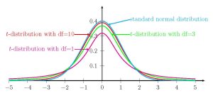
- The graph for the [latex]t[/latex]-distribution is a symmetric, bell-shaped curve, similar to the standard normal curve. The graph is symmetric about the mean 0.
- The [latex]t[/latex]-distribution has more probability in its tails than the standard normal distribution because the spread of the [latex]t[/latex]-distribution is greater than the spread of the standard normal distribution. So the graph of the [latex]t[/latex]-distribution will be thicker in the tails and shorter in the center than the graph of the standard normal distribution.
- The exact shape of the [latex]t[/latex]-distribution depends on the degrees of freedom. As the degrees of freedom increases, the graph of [latex]t[/latex]-distribution becomes more like the graph of the standard normal distribution. In fact, the [latex]t[/latex]-distribution with an infinite number of degrees of freedom is the standard normal distribution.
- The underlying population of individual observations is assumed to be normally distributed with unknown population mean [latex]\mu[/latex] and unknown population standard deviation [latex]\sigma[/latex]. The size of the underlying population is generally not relevant unless it is very small. If it is bell shaped (normal) then the assumption is met and does not need discussion. Random sampling is assumed, but that is a completely separate assumption from normality.
Constructing the Confidence Interval
When finding a confidence interval for an unknow population mean when the population standard deviation is unknown, we use the sample standard deviation [latex]s[/latex] as an estimate for the (unknown) population standard deviation and we use a [latex]t[/latex]-distribution with [latex]n-1[/latex] degrees of freedom to find the required [latex]t[/latex]-score for the confidence interval. In this case we replace the [latex]z[/latex]-score with a [latex]t[/latex]-score and [latex]\sigma[/latex] with [latex]s[/latex] in the formulas for the limits of the confidence interval for a population mean.
To construct the confidence interval, take a random sample of size [latex]n[/latex] from the population. Calculate the sample mean [latex]\overline{x}[/latex] and the sample standard deviation [latex]s[/latex]. The limits for the confidence interval with confidence level [latex]C[/latex] for an unknown population mean [latex]\mu[/latex] when the population standard deviation [latex]\sigma[/latex] is unknown are
[latex]\begin{eqnarray*} \\ \mbox{Lower Limit} & = & \overline{x}-t \times \frac{s}{\sqrt{n}} \\ \\ \mbox{Upper Limit} & = & \overline{x}+t \times \frac{s}{\sqrt{n}} \\ \\ \end{eqnarray*}[/latex]
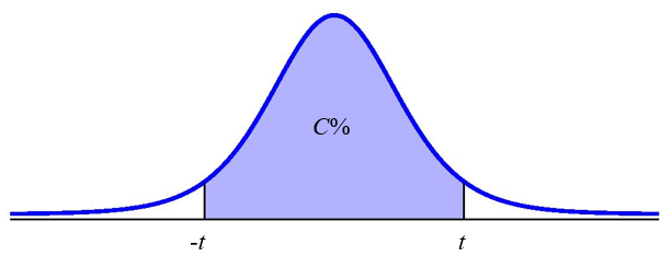
where [latex]t[/latex] is the (positive) [latex]t[/latex]-score of the [latex]t[/latex]-distribution with [latex]n-1[/latex] degrees of freedom so the area under the [latex]t[/latex]-distribution in between [latex]-t[/latex] and [latex]t[/latex] is [latex]C[/latex].
CALCULATING THE [latex]\textcolor{white}t[/latex]-SCORE FOR A CONFIDENCE INTERVAL IN EXCEL
To find the [latex]t[/latex]-score to construct a confidence interval with confidence level [latex]C[/latex], use the t.inv.2t(area in the tails, degrees of freedom) function.
- For area in the tails, enter the sum of the area in the tails of the [latex]t[/latex]-distribution. For a confidence interval, the area in the tails is [latex]1-C[/latex].
- For degrees of freedom, enter the value of the degrees of freedom for the [latex]t[/latex]-distribution. For a confidence interval for a population mean, the degrees of freedom is [latex]n-1[/latex].
The output from the t.inv.2t function is the value of the [latex]t[/latex]-score needed to construct the confidence interval.
Visit the Microsoft page for more information about the t.inv.2t function.
NOTE
The t.inv.2t function requires that we enter the sum of the area in both tails. The area in the middle of the distribution is the confidence level [latex]C[/latex], so the sum of the area in both tails is the leftover area [latex]1-C[/latex].
Watch this video: Confidence Interval for a population mean – [latex]\sigma[/latex] unknown by Joshua Emmanuel [7:40]
EXAMPLE
Suppose you do a study of acupuncture to determine how effective it is in relieving pain. You measure sensory rates for 15 subjects with the results given below.
| 8.6 | 7.3 | 10.3 |
| 9.4 | 9.2 | 5.4 |
| 7.9 | 9.6 | 8.1 |
| 6.8 | 8.7 | 5.5 |
| 8.3 | 11.4 | 6.9 |
- Construct a 95% confidence interval for the mean sensory rate.
- Interpret the confidence interval found in part 1.
- Is it reasonable to conclude that mean sensory rate is 10? Explain.
Solution:
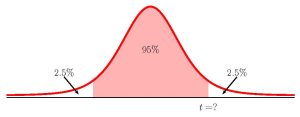
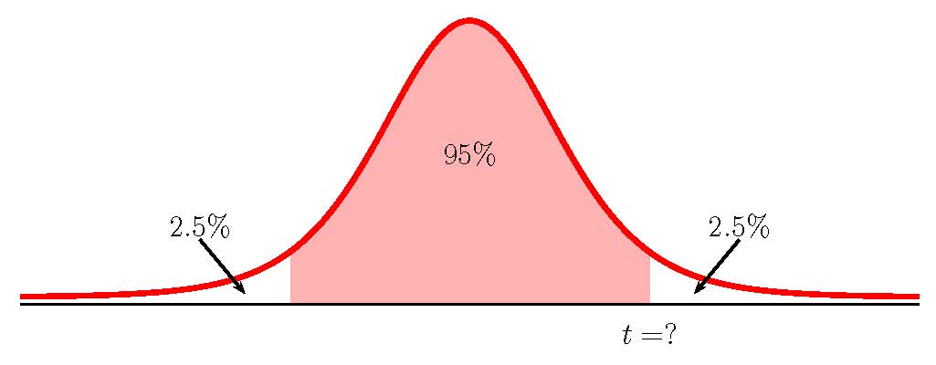
- To find the confidence interval, we need to find the [latex]t[/latex]-score for the 95% confidence interval. This means that we need to find the [latex]t[/latex]-score so that the area in the tails is [latex]1-0.95=0.05[/latex]. The degrees of freedom for the [latex]t[/latex]-distribution is [latex]n-1=15-1=14[/latex].
Function t.inv.2t Answer Field 1 0.05 2.1447… Field 2 14 So [latex]t=2.1447....[/latex]. From the sample data supplied in the question [latex]\overline{x}=8.226...[/latex], [latex]s=1.672...[/latex] and [latex]n=15[/latex]. The 95% confidence interval is
[latex]\begin{eqnarray*} \\ \mbox{Lower Limit} & = & \overline{x}-t \times \frac{s}{\sqrt{n}} \\ & = & 8.226...-2.1447... \times \frac{1.672...}{\sqrt{15}} \\ & = & 7.30 \\ \\ \mbox{Upper Limit} & = & \overline{x}+t \times \frac{s}{\sqrt{n}} \\ & = & 8.226...+2.1447... \times \frac{1.672...}{\sqrt{15}} \\ & = & 9.15 \\ \\ \end{eqnarray*}[/latex]
- We are 95% confident that the mean sensory rate is between 7.30 and 9.15.
- It is not reasonable to conclude that the mean sensory rate is 10 because 10 is outside of the confidence interval.
NOTE
When calculating the limits for the confidence interval keep all of the decimals in the [latex]t[/latex]-score and other values such as [latex]\overline{x}[/latex] and [latex]s[/latex] throughout the calculation. This will ensure that there is no round-off error in the answers. You can use Excel to do the calculation of the limits, clicking on the cells containing the [latex]t[/latex]-score, [latex]\overline{x}[/latex] and [latex]s[/latex], to ensure that all of the decimal places are used in the calculation.
TRY IT
You do a study of hypnotherapy to determine how effective it is in increasing the number of hours of sleep subjects get each night. You measure hours of sleep for 12 subjects with the following results.
| 8.2 | 8.6 | 8.9 | 9.2 |
| 9.1 | 6.9 | 9.9 | 7.5 |
| 7.7 | 11.2 | 10.1 | 10.5 |
- Construct a 97% confidence interval for the mean number of hours slept each night.
- Interpret the confidence interval found in part 1.
- Is it reasonable to assume that the mean number of hours slept each night is 9 hours? Explain.
Click to see Solution
-
Function t.inv.2t Answer Field 1 0.03 2.4906… Field 2 11 [latex]\begin{eqnarray*} \\ \mbox{Lower Limit} & = & \overline{x}-t \times \frac{s}{\sqrt{n}} \\ & = & 8.9833...-2.4906... \times \frac{1.2904...}{\sqrt{12}} \\ & = & 8.056 \\ \\ \mbox{Upper Limit} & = & \overline{x}+t \times \frac{s}{\sqrt{n}} \\ & = & 8.9833...+2.4906... \times \frac{1.2904...}{\sqrt{12}} \\ & = & 9.911 \\ \\ \end{eqnarray*}[/latex]
- We are 97% confident that the mean number of hours slept each night is between 8.056 hours and 9.911 hours.
- It is reasonable to assume the mean number of hour slept each night is 9 hours because 9 is inside the confidence interval.
EXAMPLE
The Human Toxome Project (HTP) is working to understand the scope of industrial pollution in the human body. Industrial chemicals may enter the body through pollution or as ingredients in consumer products. In October 2008, the scientists at HTP tested cord blood samples for 20 newborn infants in the United States. The cord blood of the “In utero/newborn” group was tested for 430 industrial compounds, pollutants, and other chemicals, including chemicals linked to brain and nervous system toxicity, immune system toxicity, and reproductive toxicity, and fertility problems. There are health concerns about the effects of some chemicals on the brain and nervous system. This table shows how many of the targeted chemicals were found in each infant’s cord blood.
| 79 | 145 | 147 | 160 | 116 | 100 | 159 | 151 | 156 | 126 |
| 137 | 83 | 156 | 94 | 121 | 144 | 123 | 114 | 139 | 99 |
- Construct a 90% confidence interval for the mean number of targeted industrial chemicals found in an infant’s blood.
- Interpret the confidence interval found in part 1.
Solution:
- To find the confidence interval, we need to find the [latex]t[/latex]-score for the 90% confidence interval. This means that we need to find the [latex]t[/latex]-score so that the area in the tails is [latex]1-0.90=0.1[/latex]. The degrees of freedom for the [latex]t[/latex]-distribution is [latex]n-1=20-1=19[/latex]
Function t.inv.2t Answer Field 1 0.1 1.7291… Field 2 19 So [latex]t=1.7291....[/latex]. From the sample data supplied in the question [latex]\overline{x}=127.45[/latex], [latex]s=25.9645...[/latex] and [latex]n=20[/latex]. The 90% confidence interval is
[latex]\begin{eqnarray*} \\ \mbox{Lower Limit} & = & \overline{x}-t \times \frac{s}{\sqrt{n}} \\ & = & 127.45-1.7291... \times \frac{25.9645...}{\sqrt{20}} \\ & = & 117.41 \\ \\ \mbox{Upper Limit} & = & \overline{x}+t \times \frac{s}{\sqrt{n}} \\ & = & 127.45+1.7291... \times \frac{25.9645...}{\sqrt{20}} \\ & = & 137.49 \\ \\ \end{eqnarray*}[/latex]
- We are 90% confident that the mean number of targeted industrial chemicals found in an infant’s blood is between 117.41 and 137.49.
TRY IT
A random sample of statistics students were asked to estimate the total number of hours they spend watching television in an average week. The responses are recorded in this table.
| 0 | 3 | 1 | 20 | 9 |
| 5 | 10 | 1 | 10 | 4 |
| 14 | 2 | 4 | 4 | 5 |
- Construct a 98% confidence interval for the mean number of hours statistics students will spend watching television in one week.
- Interpret the confidence interval found in part 1.
- Is it reasonable to conclude that the mean number of hours statistics students spend watching television in one week is 5? Explain.
Click to see Solution
-
Function t.inv.2t Answer Field 1 0.02 2.6244… Field 2 14  [latex]\begin{eqnarray*} \\ \mbox{Lower Limit} & = & \overline{x}-t \times \frac{s}{\sqrt{n}} \\ & = & 6.133...-2.6244... \times \frac{5.514...}{\sqrt{15}} \\ & = & 2.397 \\ \\ \mbox{Upper Limit} & = & \overline{x}+t \times \frac{s}{\sqrt{n}} \\ & = & 6.133...+2.6244... \times \frac{5.514...}{\sqrt{15}} \\ & = & 9.870 \\ \\ \end{eqnarray*}[/latex]
 - We are 98% confident that the mean number of hours statistics students will spend watching television in one week is between 2.397 hours and 9.870 hours.
- It is reasonable to assume the mean number of hours statistics students will spend watching television in one week is 5 hours because 5 is inside the confidence interval.
Concept Review
In many cases, the population standard deviation [latex]\sigma[/latex] for the population being studied is unknown. In these cases, it is common to use the sample standard deviation [latex]s[/latex] as an estimate of [latex]\sigma[/latex]. The normal distribution creates accurate confidence intervals when [latex]\sigma[/latex] is known, but it is not as accurate when [latex]s[/latex] is used as an estimate. In this case, the [latex]t[/latex]-distribution is much better.
The general form for a confidence interval for a single population mean with unknown population standard deviation is given by
[latex]\begin{eqnarray*} \\ \mbox{Lower Limit} & = & \overline{x}-t \times \frac{s}{\sqrt{n}} \\ \\ \mbox{Upper Limit} & = & \overline{x}+t \times \frac{s}{\sqrt{n}} \\ \\ \end{eqnarray*}[/latex]
where [latex]t[/latex] is the (positive) [latex]t[/latex]-score of the [latex]t[/latex]-distribution with [latex]n-1[/latex] degrees of freedom so the area under the [latex]t[/latex]-distribution in between [latex]-t[/latex] and [latex]t[/latex] is [latex]C[/latex].
Attribution
“8.2 A Single Population Mean using the Student t Distribution“ in Introductory Statistics by OpenStax is licensed under a Creative Commons Attribution 4.0 International License.
