10.5 The Test of Independence
LEARNING OBJECTIVES
- Conduct and interpret the [latex]\chi^2[/latex] test of independence.
Given two categorical variables, is there some relationship between the two categorical variables or are the two categorical variables independent. The [latex]\chi^2[/latex] test of independence allows us to test if two categorical variables are independent (not related) or dependent (related). The test of independence can only show if a relationship exists between two variables, but the test does not show if one variable causes changes in the other variable.
The test of independence uses a contingency table to analyze the data. As we saw previously in probability, a contingency table lists the categories of one variables as the rows and the categories of the other variable as the columns. The frequency of a row-column combination is the number of items that occur in both categories.
Steps to Conduct a [latex]\chi^2[/latex] Test of Independence
Suppose one categorical variable has [latex]r[/latex] possible outcomes (categories) and the other categorical variable has [latex]c[/latex] possible outcomes (categories).
- Write down the null and alternative hypotheses:
[latex]\begin{eqnarray*} \\ H_0: & &\mbox{The two categorical variables are independent}\\ H_a: & &\mbox{The two categorical variables are dependent} \\ \\ \end{eqnarray*}[/latex]
- Collect the sample information for the test and identify the significance level [latex]\alpha[/latex].
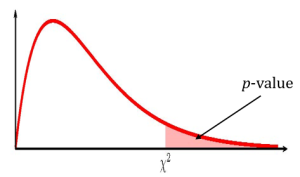
- Use the [latex]\chi^2[/latex]-distribution to find the p-value, which is the area in the right tail of the distribution. The [latex]\chi^2[/latex]-score and degrees of freedom are
[latex]\begin{eqnarray*}\chi^2 & = & \sum \frac{(\mbox{observed-expected})^2}{\mbox{expected}} \\ \\ df &= & (r-1) \times (c-1) \\ \\ \mbox{observed} & = & \mbox{observed frequency from the sample data} \\ \mbox{expected} & = & \frac{\mbox{row total} \times \mbox{column total}}{\mbox{table total}} \\ r & = & \mbox{number of rows in the contingency table} \\ c & = & \mbox{number of columns in the contingency table}\\ \\ \end{eqnarray*}[/latex]
- Compare the p-value to the significance level and state the outcome of the test:
- If p-value[latex]\leq \alpha[/latex], reject [latex]H_0[/latex] in favour of [latex]H_a[/latex].
- The results of the sample data are significant. There is sufficient evidence to conclude that the null hypothesis [latex]H_0[/latex] is an incorrect belief and that the alternative hypothesis [latex]H_a[/latex] is most likely correct.
- If p-value[latex]\gt \alpha[/latex], do not reject [latex]H_0[/latex].
- The results of the sample data are not significant. There is not sufficient evidence to conclude that the alternative hypothesis [latex]H_a[/latex] may be correct.
- If p-value[latex]\leq \alpha[/latex], reject [latex]H_0[/latex] in favour of [latex]H_a[/latex].
- Write down a concluding sentence specific to the context of the question.
NOTES
- The null hypothesis is the claim that the two categorical variables are independent. That is, there is no relationship between the two categorical variables.
- The alternative hypothesis is the claim that the two categorical variables are dependent. That is, there is some relationship between the two categorical variables.
- The test can only show if a relationship exists between the two categorical variables. The test cannot show any type of causal relationship between the two categorical variables.
- The formula to find the expected frequencies follows from the assumption that the null hypothesis is true and how we calculate joint probabilities for independent events. Assuming the null hypothesis is true means that we assume the variables are independent. This means that we assume that the events in any row and column combination of the contingency tables are independent. As we saw in probability, when two events [latex]A[/latex] and [latex]B[/latex] are independent, [latex]P(A \mbox{ and } B)=P(A) \times P(B)[/latex]. Using this fact, we get the formula for the expected frequency: [latex]\displaystyle{\mbox{expected} = \frac{\mbox{row total} \times \mbox{column total}}{\mbox{table total}}}[/latex].
- In order to use the [latex]\chi^2[/latex] test of independence, the expected frequency for a cell in the contingency table must be at least 5.
- The p-value for a [latex]\chi^2[/latex] test of independence is always the area in the right tail of the [latex]\chi^2[/latex]-distribution. So, we use chisq.dist.rt to find the p-value for a [latex]\chi^2[/latex] test of independence.
- To calculate the [latex]\chi^2[/latex]-score:
- For each of the possible outcomes of the categorical variables, calculate [latex]\displaystyle{\frac{(\mbox{observed-expected})^2}{\mbox{expected}}}[/latex]:
- Find the difference between the observed frequency (from the sample) and the expected frequency (from the null hypothesis). The expected frequency of any cell of the contingency table when the null hypothesis is true is: [latex]\displaystyle{\mbox{expected} =\frac{\mbox{row total} \times \mbox{column total}}{\mbox{table total}}}[/latex]
- Square the difference in step (i).
- Divide the value found in step (iii) by the expected frequency.
- Add up the values of [latex]\displaystyle{\frac{(\mbox{observed-expected})^2}{\mbox{expected}}}[/latex] for each of the outcomes.
- For each of the possible outcomes of the categorical variables, calculate [latex]\displaystyle{\frac{(\mbox{observed-expected})^2}{\mbox{expected}}}[/latex]:
EXAMPLE
A researcher is studying the relationship between the drivers who commit speeding violations and drivers who use cell phones while driving. The researcher took a sample of 755 drivers and obtained the information shown in the table below.
| Speeding violation in the last year | No speeding violation in the last year | Total | |
| Cell phone user | [latex]25[/latex] | [latex]280[/latex] | [latex]305[/latex] |
| Not a cell phone user | [latex]45[/latex] | [latex]405[/latex] | [latex]450[/latex] |
| Total | [latex]70[/latex] | [latex]685[/latex] | [latex]755[/latex] |
At the 5% significance level, is there a relationship between drivers who commit speeding violations and drivers who use cell phones while driving?
Solution:
Hypotheses:
[latex]\begin{eqnarray*} H_0: & & \mbox{The two variables are independent} \\ H_a: & & \mbox{The two variables are dependent} \end{eqnarray*}[/latex]
p-value:
From the question, we have [latex]r=2[/latex] and [latex]c=2[/latex]. Now we need to calculate out the [latex]\chi^2[/latex]-score for the test.
The observed frequency for each cell is the number of observations in the sample that fall into that cell. This is the information provided in the sample above.
| Observed Frequencies (Sample Data) |
|||
| Speeding violation in the last year | No speeding violation in the last year | Total | |
| Cell phone user | [latex]25[/latex] | [latex]280[/latex] | [latex]305[/latex] |
| Not a cell phone user | [latex]45[/latex] | [latex]405[/latex] | [latex]450[/latex] |
| Total | [latex]70[/latex] | [latex]685[/latex] | [latex]755[/latex] |
Next, we must calculate out the expected frequencies. Because we assume the null hypothesis is true (i.e. the variables are independent), the expected frequency in each cell is
[latex]\begin{eqnarray*} \mbox{expected} & = & \frac{\mbox{row total} \times \mbox{column total}}{\mbox{table total}} \end{eqnarray*}[/latex]
| Expected Frequencies |
|||
| Speeding violation in the last year | No speeding violation in the last year | Total | |
| Cell phone user | [latex]\displaystyle{\frac{305 \times 70}{755}=28.27...}[/latex] | [latex]\displaystyle{\frac{305 \times 685}{755}=276.72...}[/latex] | [latex]305[/latex] |
| Not a cell phone user | [latex]\displaystyle{\frac{450 \times 70}{755}=41.72...}[/latex] | [latex]\displaystyle{\frac{450\times 685}{755}=408.27...}[/latex] | [latex]450[/latex] |
| Total | [latex]70[/latex] | [latex]685[/latex] | [latex]755[/latex] |
To calculate the [latex]\chi^2[/latex]-score, for each cell we work out the quantity [latex]\displaystyle{\frac{(\mbox{observed-expected})^2}{\mbox{expected}}}[/latex] and then add up these quantities.
[latex]\begin{eqnarray*} \chi^2 & = & \sum \frac{(\mbox{observed-expected})^2}{\mbox{expected}} \\ & = & \frac{(25-28.27...)^2}{28.27...}+\frac{(280-276.72...)^2}{276.72...}+\frac{(45-41.72...)^2}{41.72...}+\frac{(405-408.27...)^2}{408.27...} \\ & = & 0.7027... \end{eqnarray*}[/latex]
The degrees of freedom for the [latex]\chi^2[/latex]-distribution is [latex]df=(r-1) \times (c-1)=(2-1) \times (2-1)=1[/latex]. The [latex]\chi^2[/latex] test of independence is a right tailed test, so the we use chisq.dist.rt function to find the p-value:
| Function | chisq.dist.rt | Answer |
| Field 1 | 0.7027…. | 0.4019 |
| Field 2 | 1 |
So the p-value[latex]=0.4019[/latex].
Conclusion:
Because p-value[latex]=0.4019 \gt 0.05=\alpha[/latex], we do not reject the null hypothesis. At the 5% significance level there is enough evidence to suggest that the two variables are independent.
NOTES
- The null hypothesis is the claim that the variables are independent. That is, there is no relationship between drivers who commit speeding violations and drivers who use cell phones while driving.
- The alternative hypothesis is the claim that the variables are dependent. That is, there is a relationship between drivers who commit speeding violations and drivers who use cell phones while driving.
- Keep all of the decimals throughout the calculation (i.e. in the calculation of the [latex]\chi^2[/latex]-score) to avoid any round-off error in the calculation of the p-value. This ensures that we get the most accurate value for the p-value.
- The p-value is the area in the right tail of the [latex]\chi^2[/latex]-distribution, to the right of [latex]\chi^2=0.7027...[/latex]. In the calculation of the p-value:
- The function is chisq.dist.rt because we are finding the area in the right tail of a [latex]\chi^2[/latex]-distribution.
- Field 1 is the value of [latex]\chi^2[/latex].
- Field 2 is the value of the degrees of freedom [latex]df[/latex].
- The p-value of 0.4019 is a large probability compared to the significance level, and so is likely to happen assuming the null hypothesis is true. This suggests that the assumption that the null hypothesis is true is most likely correct, and so the conclusion of the test is to not reject the null hypothesis. In other words, the two variables are independent.
EXAMPLE
In a volunteer group, adults 21 and older volunteer from one to nine hours each week to spend time with a disabled senior citizen. The program recruits among college students, university students, and non students. The table below is a sample of the adult volunteers and the number of hours they volunteer per week.
| 1-3 Hours | 4-6 Hours | 7-9 Hours | Total | |
| College Students | [latex]111[/latex] | [latex]96[/latex] | [latex]48[/latex] | [latex]255[/latex] |
| University Students | [latex]96[/latex] | [latex]133[/latex] | [latex]61[/latex] | [latex]290[/latex] |
| Non Students | [latex]91[/latex] | [latex]150[/latex] | [latex]53[/latex] | [latex]294[/latex] |
| Total | [latex]298[/latex] | [latex]379[/latex] | [latex]162[/latex] | [latex]839[/latex] |
At the 5% significance level, is the number of hours volunteered independent of the type of volunteer?
Solution:
Hypotheses:
[latex]\begin{eqnarray*} H_0: & & \mbox{The two variables are independent} \\ H_a: & & \mbox{The two variables are dependent} \end{eqnarray*}[/latex]
p-value:
From the question, we have [latex]r=3[/latex] and [latex]c=3[/latex]. Now we need to calculate out the [latex]\chi^2[/latex]-score for the test.
The observed frequency for each cell is the number of observations in the sample that fall into that cell. This is the information provided in the sample above.
| Observed Frequencies (Sample Data) |
||||
| 1-3 Hours | 4-6 Hours | 7-9 Hours | Total | |
| College Students | [latex]111[/latex] | [latex]96[/latex] | [latex]48[/latex] | [latex]255[/latex] |
| University Students | [latex]96[/latex] | [latex]133[/latex] | [latex]61[/latex] | [latex]290[/latex] |
| Non Students | [latex]91[/latex] | [latex]150[/latex] | [latex]53[/latex] | [latex]294[/latex] |
| Total | [latex]298[/latex] | [latex]379[/latex] | [latex]162[/latex] | [latex]839[/latex] |
Next, we must calculate out the expected frequencies. Because we assume the null hypothesis is true (i.e. the variables are independent), the expected frequency in each cell is
[latex]\begin{eqnarray*} \mbox{expected} & = & \frac{\mbox{row total} \times \mbox{column total}}{\mbox{table total}} \end{eqnarray*}[/latex]
| Expected Frequencies |
||||
| 1-3 Hours | 4-6 Hours | 7-9 Hours | Total | |
| College Students | [latex]\displaystyle{\frac{255 \times 298}{839}=90.57...}[/latex] | [latex]\displaystyle{\frac{255 \times 379}{839}=115.19...}[/latex] | [latex]\displaystyle{\frac{255 \times 162}{839}=49.23...}[/latex] | [latex]255[/latex] |
| University Students | [latex]\displaystyle{\frac{290 \times 298}{839}=103.00...}[/latex] | [latex]\displaystyle{\frac{290 \times 379}{839}=131.00...}[/latex] | [latex]\displaystyle{\frac{290 \times 162}{839}=55.99...}[/latex] | [latex]290[/latex] |
| Non Students | [latex]\displaystyle{\frac{294 \times 298}{839}=104.42...}[/latex] | [latex]\displaystyle{\frac{294 \times 379}{839}=132.80...}[/latex] | [latex]\displaystyle{\frac{294 \times 162}{839}=56.76...}[/latex] | [latex]294[/latex] |
| Total | [latex]298[/latex] | [latex]379[/latex] | [latex]162[/latex] | [latex]839[/latex] |
To calculate the [latex]\chi^2[/latex]-score, for each cell we work out the quantity [latex]\displaystyle{\frac{(\mbox{observed-expected})^2}{\mbox{expected}}}[/latex] and then add up these quantities.
[latex]\begin{eqnarray*} \chi^2 & = & \sum \frac{(\mbox{observed-expected})^2}{\mbox{expected}} \\ & = & \frac{(111-90.57...)^2}{90.57...}+\frac{(96-115.19...)^2}{115.19...}+\frac{(48-49.23...)^2}{49.23...}\\ & & +\frac{(96-103.00...)^2}{103.00...} + \frac{(133-131.00...)^2}{131.00...}+\frac{(61-55.99...)^2}{55.99...} \\ & & +\frac{(91-104.42...)^2}{104.42...}+\frac{(150-132.80...)^2}{132.80...}+ \frac{(53-56.76...)^2}{56.76...} \\ & = & 12.99... \end{eqnarray*}[/latex]
The degrees of freedom for the [latex]\chi^2[/latex]-distribution is [latex]df=(r-1) \times (c-1)=(3-1) \times (3-1)=4[/latex]. The [latex]\chi^2[/latex] test of independence is a right tailed test, so the we use chisq.dist.rt function to find the p-value:
| Function | chisq.dist.rt | Answer |
| Field 1 | 12.99…. | 0.0113 |
| Field 2 | 4 |
So the p-value[latex]=0.0113[/latex].
Conclusion:
Because p-value[latex]=0.0113 \lt 0.05=\alpha[/latex], we reject the null hypothesis in favour of the alternative hypothesis. At the 5% significance level there is enough evidence to suggest that the number of hours volunteered and type of volunteer are dependent.
NOTES
- The null hypothesis is the claim that the variables are independent. That is, there is no relationship between the number of hours volunteered and type of volunteer.
- The alternative hypothesis is the claim that the variables are dependent. That is, there is a relationship between the number of hours volunteered and type of volunteer.
- Keep all of the decimals throughout the calculation (i.e. in the calculation of the [latex]\chi^2[/latex]-score) to avoid any round-off error in the calculation of the p-value. This ensures that we get the most accurate value for the p-value.
- The p-value of 0.0113 is a small probability compared to the significance level, and so is unlikely to happen assuming the null hypothesis is true. This suggests that the assumption that the null hypothesis is true is most likely incorrect, and so the conclusion of the test is to reject the null hypothesis in favour of the alternative hypothesis. In other words, the two variables are dependent.
TRY IT
In a local school district, a music teacher wants to study the relationship between students who take music and students on the honour roll. The teacher took a sample of 300 students and obtained the information shown in the table below.
| Honour Roll Student | Non-Honour Roll Student | Total | |
| Music Student | [latex]24[/latex] | [latex]26[/latex] | [latex]50[/latex] |
| Non-Music Student | [latex]67[/latex] | [latex]183[/latex] | [latex]250[/latex] |
| Total | [latex]97[/latex] | [latex]203[/latex] | [latex]300[/latex] |
At the 5% significance level, is there a relationship between music/non-music students and honour roll/non-honour roll students?
Click to see Solution
Hypotheses:
[latex]\begin{eqnarray*} H_0: & & \mbox{The two variables are independent} \\ H_a: & & \mbox{The two variables are dependent} \end{eqnarray*}[/latex]
p-value:
From the question, we have [latex]r=2[/latex] and [latex]c=2[/latex].
| Observed Frequencies (Sample Data) |
|||
| Honour Roll Student | Non-Honour Roll Student | Total | |
| Music Student | [latex]24[/latex] | [latex]26[/latex] | [latex]50[/latex] |
| Non-Music Student | [latex]67[/latex] | [latex]183[/latex] | [latex]250[/latex] |
| Total | [latex]97[/latex] | [latex]203[/latex] | [latex]300[/latex] |
| Expected Frequencies |
|||
| Honour Roll Student | Non-Honour Roll Student | Total | |
| Music Student | [latex]16.166...[/latex] | [latex]33.833...[/latex] | [latex]50[/latex] |
| Non-Music Student | [latex]80.833...[/latex] | [latex]169.166...[/latex] | [latex]250[/latex] |
| Total | [latex]97[/latex] | [latex]203[/latex] | [latex]300[/latex] |
[latex]\begin{eqnarray*} \chi^2 & = & \sum \frac{(\mbox{observed-expected})^2}{\mbox{expected}} \\ & = & \frac{(24-16.166...)^2}{16.166...}+\frac{(26-33.833...)^2}{33.833...}+\frac{(67-80.833...)^2}{80.833...}+\frac{(183-169.166...)^2}{169.166...} \\ & = & 9.107... \\ \\ df & = & (r-1) \times (c-1) \\ & = & (2-1) \times (2-1) \\ & = & 1 \end{eqnarray*}[/latex]
| Function | chisq.dist.rt | Answer |
| Field 1 | 9.107… | 0.0025 |
| Field 2 | 1 |
So the p-value[latex]=0.0025[/latex].
Conclusion:
Because p-value[latex]=0.0025 \lt 0.05=\alpha[/latex], we reject the null hypothesis in favour of the alternative hypothesis. At the 5% significance level there is enough evidence to suggest that the two variables are dependent.
TRY IT
A local college is interested in the relationship between student anxiety level and the need to succeed in school. A random sample of 400 students took a test that measured anxiety level and the need to succeed in school. The results are shown in the table below.
| High Anxiety | Med-High Anxiety | Medium Anxiety | Med-Low Anxiety | Low Anxiety | Total | |
| High Need | [latex]35[/latex] | [latex]42[/latex] | [latex]53[/latex] | [latex]15[/latex] | [latex]10[/latex] | [latex]155[/latex] |
| Medium Need | [latex]18[/latex] | [latex]48[/latex] | [latex]63[/latex] | [latex]33[/latex] | [latex]31[/latex] | [latex]193[/latex] |
| Low Need | [latex]4[/latex] | [latex]5[/latex] | [latex]11[/latex] | [latex]15[/latex] | [latex]17[/latex] | [latex]52[/latex] |
| Total | [latex]57[/latex] | [latex]95[/latex] | [latex]127[/latex] | [latex]63[/latex] | [latex]58[/latex] | [latex]400[/latex] |
At the 5% significance level, is there a relationship between student anxiety level and the need to succeed in school?
Click to see Solution
Hypotheses:
[latex]\begin{eqnarray*} H_0: & & \mbox{The two variables are independent} \\ H_a: & & \mbox{The two variables are dependent} \end{eqnarray*}[/latex]
p-value:
From the question, we have [latex]r=3[/latex] and [latex]c=5[/latex].
| Observed Frequencies (Sample Data) |
||||||
| High Anxiety | Med-High Anxiety | Medium Anxiety | Med-Low Anxiety | Low Anxiety | Total | |
| High Need | [latex]35[/latex] | [latex]42[/latex] | [latex]53[/latex] | [latex]15[/latex] | [latex]10[/latex] | [latex]155[/latex] |
| Medium Need | [latex]18[/latex] | [latex]48[/latex] | [latex]63[/latex] | [latex]33[/latex] | [latex]31[/latex] | [latex]193[/latex] |
| Low Need | [latex]4[/latex] | [latex]5[/latex] | [latex]11[/latex] | [latex]15[/latex] | [latex]17[/latex] | [latex]52[/latex] |
| Total | [latex]57[/latex] | [latex]95[/latex] | [latex]127[/latex] | [latex]63[/latex] | [latex]58[/latex] | [latex]400[/latex] |
| Expected Frequencies |
||||||
| High Anxiety | Med-High Anxiety | Medium Anxiety | Med-Low Anxiety | Low Anxiety | Total | |
| High Need | [latex]22.08...[/latex] | [latex]36.81...[/latex] | [latex]49.21...[/latex] | [latex]24.41...[/latex] | [latex]22.47...[/latex] | [latex]155[/latex] |
| Medium Need | [latex]27.50...[/latex] | [latex]45.83...[/latex] | [latex]61.27...[/latex] | [latex]30.39...[/latex] | [latex]27.98...[/latex] | [latex]193[/latex] |
| Low Need | [latex]7.41[/latex] | [latex]12.35[/latex] | [latex]16.51[/latex] | [latex]8.19[/latex] | [latex]7.54[/latex] | [latex]52[/latex] |
| Total | [latex]57[/latex] | [latex]95[/latex] | [latex]127[/latex] | [latex]63[/latex] | [latex]58[/latex] | [latex]400[/latex] |
[latex]\begin{eqnarray*} \chi^2 & = & \sum \frac{(\mbox{observed-expected})^2}{\mbox{expected}} \\ & = & \frac{(35-22.08...)^2}{22.08...}+\frac{(18-27.50...)^2}{27.50...}+\frac{(4-7.41)^2}{7.41} \\ & & +\frac{(42-36.81...)^2}{36.81...}+\frac{(48-45.83...)^2}{45.83...}+\frac{(5-12.35)^2}{12.35} \\ & & +\frac{(53-49.21...)^2}{49.21...}+\frac{(63-61.27...)^2}{61.27...}+\frac{(11-16.51)^2}{16.51} \\ & & +\frac{(15-24.41...)^2}{24.41...}+\frac{(33-30.39...)^2}{30.39...}+\frac{(15-8.19)^2}{8.19} \\ & & +\frac{(10-22.47...)^2}{22.47...}+\frac{(31-27.98...)^2}{27.98...}+\frac{(17-7.54)^2}{7.54} \\ & = & 48.419... \\ \\ df & = & (r-1) \times (c-1) \\ & = & (3-1) \times (5-1) \\ & = & 8 \end{eqnarray*}[/latex]
| Function | chisq.dist.rt | Answer |
| Field 1 | 48.419… | 0.00000008 |
| Field 2 | 8 |
So the p-value[latex]=0.00000008[/latex].
Conclusion:
Because p-value[latex]=0.00000008 \lt 0.05=\alpha[/latex], we reject the null hypothesis in favour of the alternative hypothesis. At the 5% significance level there is enough evidence to suggest that the two variables are dependent.
Watch this video: Chi-Square Test of Independence by Khan Academy [10:27]
Concept Review
The [latex]\chi^2[/latex] test of independence is used to determine if two categorical variables are independent or dependent. The test of independence is a well established process:
- Write down the null and alternative hypotheses. The null hypothesis is the claim that the categorical variables are independent and the alternative hypothesis is the claim that the categorical variables are dependent.
- Collect the sample information for the test and identify the significance level.
- The p-value is the area in the right tail of the [latex]\chi^2[/latex]-distribution where [latex]\displaystyle{\chi^2 = \sum \frac{(\mbox{observed-expected})^2}{\mbox{expected}}}[/latex] and [latex]df=(r-1) \times (c-1)[/latex].
- Compare the p-value to the significance level and state the outcome of the test.
- Write down a concluding sentence specific to the context of the question.
Attribution
“11.3 Test of Independence“ in Introductory Statistics by OpenStax is licensed under a Creative Commons Attribution 4.0 International License.
