13.3 Standard Error of the Estimate
LEARNING OBJECTIVES
- Calculate and interpret the standard error of the estimate for multiple regression.
The difference between the actual value of the dependent variable [latex]y[/latex] (in the sample date) and the predicted value of the dependent variable [latex]\hat{y}[/latex] obtained from the multiple regression model is called the error or residual.
[latex]\begin{eqnarray*} \mbox{Error} & = & \mbox{Actual Value}-\mbox{Predicted Value}\end{eqnarray*}[/latex]
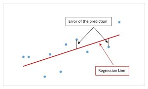
For the simple linear regression model, the standard error of the estimate measures the average vertical distance (the error) between the points on the scatter diagram and the regression line.
The standard error of the estimate, denoted [latex]s_e[/latex], is a measure of the standard deviation of the errors in a regression model. The standard error of the estimate is a measure of the average deviation of the errors, the difference between the [latex]\hat{y}[/latex]-values predicted by the multiple regression model and the [latex]y[/latex]-values in the sample. The standard error of the estimate for the regression model is the standard deviation of the errors/residuals.
The value of [latex]s_e[/latex] tells us, on average, how much the dependent variable differs from the regression model based on the independent variables. When interpreting the standard error of the estimate, remember to be specific to the question, using the actual names of the dependent and independent variables, and include appropriate units. The units of the standard error of the estimate are the same as the units of the dependent variable.
The value of the standard error of the estimate for the regression model can be found on the regression summary table, which we learned how to generate in Excel in the previous section.
EXAMPLE
The human resources department at a large company wants to develop a model to predict an employee’s job satisfaction from the number of hours of unpaid work per week the employee does, the employee’s age, and the employee’s income. A sample of 25 employees at the company is taken and the data is recorded in the table below. The employee’s income is recorded in $1000s and the job satisfaction score is out of 10, with higher values indicating greater job satisfaction.
| Job Satisfaction | Hours of Unpaid Work per Week | Age | Income ($1000s) |
| 4 | 3 | 23 | 60 |
| 5 | 8 | 32 | 114 |
| 2 | 9 | 28 | 45 |
| 6 | 4 | 60 | 187 |
| 7 | 3 | 62 | 175 |
| 8 | 1 | 43 | 125 |
| 7 | 6 | 60 | 93 |
| 3 | 3 | 37 | 57 |
| 5 | 2 | 24 | 47 |
| 5 | 5 | 64 | 128 |
| 7 | 2 | 28 | 66 |
| 8 | 1 | 66 | 146 |
| 5 | 7 | 35 | 89 |
| 2 | 5 | 37 | 56 |
| 4 | 0 | 59 | 65 |
| 6 | 2 | 32 | 95 |
| 5 | 6 | 76 | 82 |
| 7 | 5 | 25 | 90 |
| 9 | 0 | 55 | 137 |
| 8 | 3 | 34 | 91 |
| 7 | 5 | 54 | 184 |
| 9 | 1 | 57 | 60 |
| 7 | 0 | 68 | 39 |
| 10 | 2 | 66 | 187 |
| 5 | 0 | 50 | 49 |
Previously, we found the multiple regression equation to predict the job satisfaction score from the other variables:
[latex]\begin{eqnarray*} \hat{y} & = & 4.7993-0.3818x_1+0.0046x_2+0.0233x_3 \\ \\ \hat{y} & = & \mbox{predicted job satisfaction score} \\ x_1 & = & \mbox{hours of unpaid work per week} \\ x_2 & = & \mbox{age} \\ x_3 & = & \mbox{income (\$1000s)}\end{eqnarray*}[/latex]
- Find the standard error of the estimate.
- Interpret the standard error of the estimate.
Solution:
- The regression summary table generated by Excel is shown below:
SUMMARY OUTPUT Regression Statistics Multiple R 0.711779225 R Square 0.506629665 Adjusted R Square 0.436148189 Standard Error 1.585212784 Observations 25 ANOVA df SS MS F Significance F Regression 3 54.189109 18.06303633 7.18812504 0.001683189 Residual 21 52.770891 2.512899571 Total 24 106.96 Coefficients Standard Error t Stat P-value Lower 95% Upper 95% Intercept 4.799258185 1.197185164 4.008785216 0.00063622 2.309575344 7.288941027 Hours of Unpaid Work per Week -0.38184722 0.130750479 -2.9204269 0.008177146 -0.65375772 -0.10993671 Age 0.004555815 0.022855709 0.199329423 0.843922453 -0.04297523 0.052086864 Income ($1000s) 0.023250418 0.007610353 3.055103771 0.006012895 0.007423823 0.039077013 The standard error of the estimate for the regression models is in the top part of the table, under the Regression Statistics heading in the Standard Error row. The value of the standard error of the estimate is [latex]s_e=1.5852[/latex].
- On average, the job satisfaction score is 1.5852 points away from the regression model based on the independent variables “hours of unpaid work per week,” “age,” and “income.”
NOTE
The standard error of the estimate for the regression model is located in the top part of the table under the Regression Statistics heading. You will notice another standard error column at the bottom in the rows corresponding to the independent variables. These standard errors in the bottom part of the table are not related to the standard error of the estimate. In fact, the standard errors in the independent variable rows are measures of the uncertainty around the estimate of the regression coefficient for each independent variable.
Concept Review
The standard error of the estimate, [latex]s_e[/latex], measures the average deviation of the errors of the regression model. The smaller the value of the standard error of the estimate, the better the fit of the regression model to the data.
