12.7 Standard Error of the Estimate
LEARNING OBJECTIVES
- Calculate and interpret the standard error of the estimate.
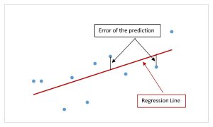
The difference between the actual value of the dependent variable [latex]y[/latex] (in the sample data) and the predicted value of the dependent variable [latex]\hat{y}[/latex] obtained from the linear regression equation is called the error or residual.
[latex]\begin{eqnarray*} \mbox{Error} & = & \mbox{Actual Value}-\mbox{Predicted Value}\end{eqnarray*}[/latex]
Graphically, the absolute value of the error is the vertical distance between the actual value of [latex]y[/latex] (the point on the scatter diagram) and the predicted value of [latex]\hat{y}[/latex] (the point on the linear regression line). In other words, the absolute value of the error measures the vertical distance between the actual data point and the line.
The standard error of the estimate, denoted [latex]s_e[/latex], is a measure of the standard deviation of the errors in a regression model. The standard error of the estimate is a measure of the average deviation or dispersion of the points on the scatter diagram around the line-of-best-fit. The standard error of the estimate for the linear regression model is analogous to the standard deviation for a set of points, but instead of measuring the average distance from the mean we are measuring the average distance from the regression line. Graphically, the standard error of the estimate measures the average vertical distance (the absolute value of the errors) between the points on the scatter diagram and the regression line.
When the points on the scatter diagram are close to the regression line, the errors are small, and so the average of the dispersion of the points around the line will be small. In this case, the value of the standard error of the estimate will be relatively small, which reflects the fact that there is little variation between the actual data pints (the points on the scatter diagram) and the linear regression model. This implies that the linear regression model is a good fit for the data and predictions made with the linear regression model will be fairly accurate.
Conversely, when the points on the scatter diagram are widely dispersed around the regression line, there errors are large, and so the average dispersion of the points around the line will be large. In this case, the value of the standard error of the estimate will be large, which reflects the greater dispersion between the actual data points and the linear regression model. This implies that the linear regression model is not a good fit for the data and predictions made with the linear regression model will be inaccurate.
The value of [latex]s_e[/latex] tells us, on average, how much the dependent variable differs from the regression line based on the independent variable. When interpreting the standard error of the estimate, remember to be specific to the question, using the actual names of the dependent and independent variables, and include appropriate units. The units of the standard error of the estimate are the same as the units of the dependent variable.
Although there is a formula to calculate out the value of the standard error of the estimate, we will calculate the standard error of the estimate using the built-in function in Excel.
CALCULATING THE STANDARD ERROR OF THE ESTIMATE IN EXCEL
To calculate the standard error of the estimate, use the steyx(array for y’s,array for x’s) function.
- For array for y’s, enter the cell array containing the dependent variable [latex]y[/latex] data.
- For array for x’s, enter the cell array containing the independent variable [latex]x[/latex] data.
Visit the Microsoft page for more information about the steyx function.
NOTE
The order in which the data is entered into the steyx function is important. The data for the dependent variable is entered in the first array and the data for the independent variable is entered in the second array. The output from the steyx function will be different when the order of the inputs is switched.
EXAMPLE
A statistics professor wants to study the relationship between a student’s score on the third exam in the course and their final exam score. The professor took a random sample of 11 students and recorded their third exam score (out of 80) and their final exam score (out of 200). The results are recorded in the table below. The professor wants to develop a linear regression model to predict a student’s final exam score from the third exam score.
| Student | Third Exam Score | Final Exam Score |
| 1 | 65 | 175 |
| 2 | 67 | 133 |
| 3 | 71 | 185 |
| 4 | 71 | 163 |
| 5 | 66 | 126 |
| 6 | 75 | 198 |
| 7 | 67 | 153 |
| 8 | 70 | 163 |
| 9 | 71 | 159 |
| 10 | 69 | 151 |
| 11 | 69 | 159 |
Previously we found the line-of-best-fit [latex]\hat{y}=-173.51+4.83x[/latex] where [latex]x[/latex] is the third exam score and [latex]\hat{y}[/latex] is the (predicted) final exam score.
- Find the standard error of the estimate.
- Interpret the standard error of the estimate found in part 1.
Solution:
- Enter the data into an Excel spreadsheet. For this example, suppose we entered the data (without the column headings) so that the student column is in column A from A1 to A11, the third exam score is in column B from B1 to B11, and the final exam score is in column C from C1 to C11.
Function steyx Answer Field 1 C1:C11 16.41 Field 2 B1:B11 The value of the standard error of the estimate is [latex]s_e=16.41[/latex].
- On average, the final exam score differs by 16.41 points from the regression line based on the third exam score.
TRY IT
SCUBA divers have maximum dive times they cannot exceed when going to different depths. The data in the table below shows different depths with the maximum dive times in minutes. Previously we found the regression line to predict the maximum dive time from depth.
| Depth (in feet) | Maximum Dive Time (in minutes) |
| 50 | 80 |
| 60 | 55 |
| 70 | 45 |
| 80 | 35 |
| 90 | 25 |
| 100 | 22 |
- Find the standard error of the estimate.
- Interpret the standard error of the estimate found in part 1.
Click to see Solution
- [latex]\displaystyle{s_e=6.53}[/latex].
- On average, the maximum dive time differs by 6.53 minutes from the regression line based on depth.
Concept Review
The standard error of the estimate, [latex]s_e[/latex], measures the average deviation or dispersion of the points on the scatter diagram around the line-of-best-fit. The smaller the value of the standard error of the estimate, the better the fit of the regression line to the data.
