8.8 Hypothesis Tests for a Population Proportion
LEARNING OBJECTIVES
- Conduct and interpret hypothesis tests for a population proportion.
Some notes about conducting a hypothesis test:
- The null hypothesis [latex]H_0[/latex] is always an “equal to.” The null hypothesis is the original claim about the population parameter.
- The alternative hypothesis [latex]H_a[/latex] is a “less than,” “greater than,” or “not equal to.” The form of the alternative hypothesis depends on the context of the question.
- The form of the alternative hypothesis tell us if the test is left-tail, right-tail, or two-tail. The alternative hypothesis is the key to conducting the test and finding the correct p-value.
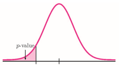
- If the alternative hypothesis is a “less than”, then the test is left-tail. The p-value is the area in the left-tail of the distribution.
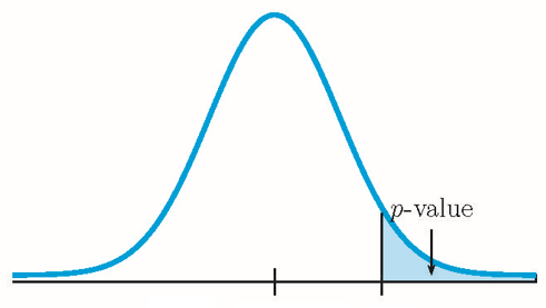
- If the alternative hypothesis is a “greater than”, then the test is right-tail. The p-value is the area in the right-tail of the distribution.
- If the alternative hypothesis is a “not equal to”, then the test is two-tail. The p-value is the sum of the area in the two-tails of the distribution. Each tail represents exactly half of the p-value.
- Think about the meaning of the p-value. A data analyst (and anyone else) should have more confidence that they made the correct decision to reject the null hypothesis with a smaller p-value (for example, 0.001 as opposed to 0.04) even if using a significance level of 0.05. Similarly, for a large p-value such as 0.4, as opposed to a p-value of 0.056 (a significance level of 0.05 is less than either number), a data analyst should have more confidence that they made the correct decision in not rejecting the null hypothesis. This makes the data analyst use judgment rather than mindlessly applying rules.
- The significance level must be identified before collecting the sample data and conducting the test. Generally, the significance level will be included in the question. If no significance level is given, a common standard is to use a significance level of 5%.
EXAMPLE
Suppose the hypotheses for a hypothesis test are:
[latex]\begin{eqnarray*} H_0: & & p=20 \% \\ H_a: & & p \gt 20\% \end{eqnarray*}[/latex]
Because the alternative hypothesis is a [latex]\gt[/latex], this is a right-tail test. The p-value is the area in the right-tail of the distribution.

EXAMPLE
Suppose the hypotheses for a hypothesis test are:
[latex]\begin{eqnarray*} H_0: & & p=50 \% \\ H_a: & & p \neq 50\% \end{eqnarray*}[/latex]
Because the alternative hypothesis is a [latex]\neq[/latex], this is a two-tail test. The p-value is the sum of the areas in the two tails of the distribution. Each tail contains exactly half of the p-value.

EXAMPLE
Suppose the hypotheses for a hypothesis test are:
[latex]\begin{eqnarray*} H_0: & & p=10\% \\ H_a: & & p \lt 10\% \end{eqnarray*}[/latex]
Because the alternative hypothesis is a [latex]\lt[/latex], this is a left-tail test. The p-value is the area in the left-tail of the distribution.
Steps to Conduct a Hypothesis Test for a Population Proportion
- Write down the null and alternative hypotheses in terms of the population proportion [latex]p[/latex]. Include appropriate units with the values of the proportion.
- Use the form of the alternative hypothesis to determine if the test is left-tailed, right-tailed, or two-tailed.
- Collect the sample information for the test and identify the significance level.
- Find the p-value (the area in the corresponding tail) for the test using the appropriate distribution:
- If [latex]n \times p \geq 5[/latex] and [latex]n \times (1-p) \geq 5[/latex], use the normal distribution with [latex]\displaystyle{z=\frac{\hat{p}-p}{\sqrt{\frac{p \times (1-p)}{n}}}}[/latex].
- If one of [latex]n \times p \lt 5[/latex] or [latex]n \times (1-p) \lt 5[/latex], use a binomial distribution.
- Compare the p-value to the significance level and state the outcome of the test:
- If p-value[latex]\leq \alpha[/latex], reject [latex]H_0[/latex] in favour of [latex]H_a[/latex].
- The results of the sample data are significant. There is sufficient evidence to conclude that the null hypothesis [latex]H_0[/latex] is an incorrect belief and that the alternative hypothesis [latex]H_a[/latex] is most likely correct.
- If p-value[latex]\gt \alpha[/latex], do not reject [latex]H_0[/latex].
- The results of the sample data are not significant. There is not sufficient evidence to conclude that the alternative hypothesis [latex]H_a[/latex] may be correct.
- If p-value[latex]\leq \alpha[/latex], reject [latex]H_0[/latex] in favour of [latex]H_a[/latex].
- Write down a concluding sentence specific to the context of the question.
USING EXCEL TO CALCULE THE P-VALUE FOR A HYPOTHESIS TEST ON A POPULATION PROPORTION
The p-value for a hypothesis test on a population proportion is the area in the tail(s) of distribution of the sample proportion. If both [latex]n \times p \geq 5[/latex] and [latex]n \times (1-p) \geq 5[/latex], use the normal distribution to find the p-value. If at least one of [latex]n \times p \lt 5[/latex] or [latex]n \times (1-p) \lt 5[/latex], use the binomial distribution to find the p-value.
If both [latex]n \times p \geq 5[/latex] and [latex]n \times (1-p) \geq 5[/latex]:
- The p-value is the area in the tail(s) of a normal distribution, so the norm.dist(x,[latex]\mu[/latex],[latex]\sigma[/latex],logic operator) function can be used to calculate the p-value.
- For x, enter the value for [latex]\hat{p}[/latex].
- For [latex]\mu[/latex], enter the mean of the sample proportions [latex]p[/latex]. Note: Because the test is run assuming the null hypothesis is true, the value for [latex]p[/latex] is the claim from the null hypothesis.
- For [latex]\sigma[/latex], enter the standard error of the proportions [latex]\displaystyle{\sqrt{\frac{p \times (1-p)}{n}}}[/latex].
- For the logic operator, enter true. Note: Because we are calculating the area under the curve, we always enter true for the logic operator.
- Use the appropriate technique with the norm.dist function to find the area in the left-tail or the area in the right-tail.
If at least one of [latex]n \times p \lt 5[/latex] or [latex]n \times (1-p) \lt 5[/latex]:
- The p-value is found using the binomial distribution.
- If the alternative hypothesis is a [latex]\lt[/latex], the p-value is the probability of getting at most [latex]x[/latex] successes in [latex]n[/latex]trials where the probability of success is the claim about the population proportion [latex]p[/latex] in the null hypothesis.
- The p-value is the output from the binom.dist(x,n,p,logic operator) function:
- For x, enter the number of successes.
- For n, enter the sample size.
- For p, enter the the value of the population proportion [latex]p[/latex] from the null hypothesis.
- For the logic operator, enter true. Note: Because we are calculating an at most probability, the logic operator is always true.
- The p-value is the output from the binom.dist(x,n,p,logic operator) function:
- If the alternative hypothesis is a [latex]\gt[/latex], the p-value is the probability of getting at least [latex]x[/latex] successes in [latex]n[/latex] trials where the probability of success is the claim about the population proportion [latex]p[/latex] in the null hypothesis.
- The p-value is the output from the 1-binom.dist(x-1,n,p,logic operator) function:
- For x, enter the number of successes.
- For n, enter the sample size.
- For p, enter the the value of the population proportion [latex]p[/latex] in the null hypothesis.
- For the logic operator, enter true. Note: Because we are calculating an at least probability, the logic operator is always true.
- The p-value is the output from the 1-binom.dist(x-1,n,p,logic operator) function:
EXAMPLE
Marketers believe that 92% of adults own a cell phone. A cell phone manufacturer believes that number is actually lower. In a sample of 200 adults, 87% own a cell phone. At the 1% significance level, determine if the proportion of adults that own a cell phone is lower than the marketers’ claim.
Solution:
Hypotheses:
[latex]\begin{eqnarray*} H_0: & & p=92\% \mbox{ of adults own a cell phone} \\ H_a: & & p \lt 92\% \mbox{ of adults own a cell phone} \end{eqnarray*}[/latex]
p-value:
From the question, we have [latex]n=200[/latex], [latex]\hat{p}=0.87[/latex], and [latex]\alpha=0.01[/latex].
To determine the distribution, we check [latex]n \times p[/latex] and [latex]n \times (1-p)[/latex]. For the value of [latex]p[/latex], we use the claim from the null hypothesis ([latex]p=0.92[/latex]).
[latex]\begin{eqnarray*} n \times p & = & 200 \times 0.92=184 \geq 5 \\ n \times (1-p) & = & 200 \times (1-0.92)=16 \geq 5\end{eqnarray*}[/latex]
Because both [latex]n \times p \geq 5[/latex] and [latex]n \times (1-p) \geq 5[/latex] we use a normal distribution to calculate the p-value. Because the alternative hypothesis is a [latex]\lt[/latex], the p-value is the area in the left tail of the distribution.
| Function | norm.dist | Answer |
| Field 1 | 0.87 | 0.0046 |
| Field 2 | 0.92 | |
| Field 3 | sqrt(0.92*(1-0.92)/200) | |
| Field 4 | true |
So the p-value[latex]=0.0046[/latex].
Conclusion:
Because p-value[latex]=0.0046 \lt 0.01=\alpha[/latex], we reject the null hypothesis in favour of the alternative hypothesis. At the 1% significance level there is enough evidence to suggest that the proportion of adults who own a cell phone is lower than 92%.
NOTES
- The null hypothesis [latex]p=92\%[/latex] is the claim that 92% of adults own a cell phone.
- The alternative hypothesis [latex]p \lt 92\%[/latex] is the claim that less than 92% of adults own a cell phone.
- The p-value is the area in the left tail of the sampling distribution, to the left of [latex]\hat{p}=0.87[/latex]. In the calculation of the p-value:
- The function is norm.dist because we are finding the area in the left tail of a normal distribution.
- Field 1 is the value of [latex]\hat{p}[/latex].
- Field 2 is the value of [latex]p[/latex] from the null hypothesis. Remember, we run the test assuming the null hypothesis is true, so that means we assume [latex]p=0.92[/latex].
- Field 3 is the standard deviation for the sample proportions [latex]\displaystyle{\sqrt{\frac{p \times (1-p)}{n}}}[/latex].
- The p-value of 0.0046 tells us that under the assumption that 92% of adults own a cell phone (the null hypothesis), there is only a 0.46% chance that the proportion of adults who own a cell phone in a sample of 200 is 87% or less. This is a small probability, and so is unlikely to happen assuming the null hypothesis is true. This suggests that the assumption that the null hypothesis is true is most likely incorrect, and so the conclusion of the test is to reject the null hypothesis in favour of the alternative hypothesis. In other words, the proportion of adults who own a cell phone is most likely less than 92%.
EXAMPLE
A consumer group claims that the proportion of households that have at least three cell phones is 30%. A cell phone company has reason to believe that the proportion of households with at least three cell phones is much higher. Before they start a big advertising campaign based on the proportion of households that have at least three cell phones, they want to test their claim. Their marketing people survey 150 households with the result that 54 of the households have at least three cell phones. At the 1% significance level, determine if the proportion of households that have at least three cell phones is less than 30%.
Solution:
Hypotheses:
[latex]\begin{eqnarray*} H_0: & & p=30\% \mbox{ of household have at least 3 cell phones} \\ H_a: & & p \gt 30\% \mbox{ of household have at least 3 cell phones} \end{eqnarray*}[/latex]
p-value:
From the question, we have [latex]n=150[/latex], [latex]\displaystyle{\hat{p}=\frac{54}{150}=0.36}[/latex], and [latex]\alpha=0.01[/latex].
To determine the distribution, we check [latex]n \times p[/latex] and [latex]n \times (1-p)[/latex]. For the value of [latex]p[/latex], we use the claim from the null hypothesis ([latex]p=0.3[/latex]).
[latex]\begin{eqnarray*} n \times p & = & 150 \times 0.3=45 \geq 5 \\ n \times (1-p) & = & 150 \times (1-0.3)=105 \geq 5\end{eqnarray*}[/latex]
Because both [latex]n \times p \geq 5[/latex] and [latex]n \times (1-p) \geq 5[/latex] we use a normal distribution to calculate the p-value. Because the alternative hypothesis is a [latex]\gt[/latex], the p-value is the area in the right tail of the distribution.
| Function | 1-norm.dist | Answer |
| Field 1 | 0.36 | 0.0544 |
| Field 2 | 0.3 | |
| Field 3 | sqrt(0.3*(1-0.3)/150) | |
| Field 4 | true |
So the p-value[latex]=0.0544[/latex].
Conclusion:
Because p-value[latex]=0.0544 \gt 0.01=\alpha[/latex], we do not reject the null hypothesis. At the 1% significance level there is not enough evidence to suggest that the proportion of households with at least three cell phones is more than 30%.
NOTES
- The null hypothesis [latex]p=30\%[/latex] is the claim that 30% of households have at least three cell phones.
- The alternative hypothesis [latex]p \gt 30\%[/latex] is the claim that more than 30% of households have at least three cell phones.
- The p-value is the area in the right tail of the sampling distribution, to the right of [latex]\hat{p}=0.36[/latex]. In the calculation of the p-value:
- The function is 1-norm.dist because we are finding the area in the right tail of a normal distribution.
- Field 1 is the value of [latex]\hat{p}[/latex].
- Field 2 is the value of [latex]p[/latex] from the null hypothesis. Remember, we run the test assuming the null hypothesis is true, so that means we assume [latex]p=0.3[/latex].
- Field 3 is the standard deviation for the sample proportions [latex]\displaystyle{\sqrt{\frac{p \times (1-p)}{n}}}[/latex].
- The p-value of 0.0544 tells us that under the assumption that 30% of households have at least three cell phones (the null hypothesis), there is a 5.44% chance that the proportion of households with at least three cell phones in a sample of 150 is 36% or more. Compared to the 1% significance level, this is a large probability, and so is likely to happen assuming the null hypothesis is true. This suggests that the assumption that the null hypothesis is true is most likely correct, and so the conclusion of the test is to not reject the null hypothesis. In other words, the claim that 30% of households have at least three cell phones is most likely correct.
TRY IT
A teacher believes that 70% of students in the class will want to go on a field trip to the local zoo. The students in the class believe the proportion is much higher and ask the teacher to verify her claim. The teacher samples 50 students and 39 reply that they would want to go to the zoo. At the 5% significance level, determine if the proportion of students who want to go on the field trip is higher than 70%.
Click to see Solution
Hypotheses:
[latex]\begin{eqnarray*} H_0: & & p = 70\% \mbox{ of students want to go on the field trip} \\ H_a: & & p \gt 70\% \mbox{ of students want to go on the field trip} \end{eqnarray*}[/latex]
p-value:
From the question, we have [latex]n=50[/latex], [latex]\displaystyle{\hat{p}=\frac{39}{50}=0.78}[/latex], and [latex]\alpha=0.05[/latex].
[latex]\begin{eqnarray*} n \times p & = & 50 \times 0.7=35 \geq 5 \\ n \times (1-p) & = & 50 \times (1-0.7)=15 \geq 5\end{eqnarray*}[/latex]
Because both [latex]n \times p \geq 5[/latex] and [latex]n \times (1-p) \geq 5[/latex] we use a normal distribution to calculate the p-value. Because the alternative hypothesis is a [latex]\gt[/latex], the p-value is the area in the right tail of the distribution.
| Function | 1-norm.dist | Answer |
| Field 1 | 0.78 | 0.1085 |
| Field 2 | 0.7 | |
| Field 3 | sqrt(0.7*(1-0.7)/50) | |
| Field 4 | true |
So the p-value[latex]=0.1085[/latex].
Conclusion:
Because p-value[latex]=0.1085 \gt 0.05=\alpha[/latex], we do not reject the null hypothesis. At the 5% significance level there is not enough evidence to suggest that the proportion of students who want to go on the field trip is higher than 70%.
NOTES
- The null hypothesis [latex]p=70\%[/latex] is the claim that 70% of the students want to go on the field trip.
- The alternative hypothesis [latex]p \gt 70\%[/latex] is the claim that more than 70% of students want to go on the field trip.
- The p-value of 0.1085 tells us that under the assumption that 70% of students want to go on the field trip (the null hypothesis), there is a 10.85% chance that the proportion of students who want to go on the field trip in a sample of 50 students is 78% or more. Compared to the 5% significance level, this is a large probability, and so is likely to happen assuming the null hypothesis is true. This suggests that the assumption that the null hypothesis is true is most likely correct, and so the conclusion of the test is to not reject the null hypothesis. In other words, the teacher’s claim that 70% of students want to go on the field trip is most likely correct.
EXAMPLE
Joan believes that 50% of first-time brides in the United States are younger than their grooms. She performs a hypothesis test to determine if the percentage is the same or different from 50%. Joan samples 100 first-time brides and 56 reply that they are younger than their grooms. Use a 5% significance level.
Solution:
Hypotheses:
[latex]\begin{eqnarray*} H_0: & & p=50\% \mbox{ of first-time brides are younger than the groom} \\ H_a: & & p \neq 50\% \mbox{ of first-time brides are younger than the groom} \end{eqnarray*}[/latex]
p-value:
From the question, we have [latex]n=100[/latex], [latex]\displaystyle{\hat{p}=\frac{56}{100}=0.56}[/latex], and [latex]\alpha=0.05[/latex].
To determine the distribution, we check [latex]n \times p[/latex] and [latex]n \times (1-p)[/latex]. For the value of [latex]p[/latex], we use the claim from the null hypothesis ([latex]p=0.5[/latex]).
[latex]\begin{eqnarray*} n \times p & = & 100 \times 0.5=50 \geq 5 \\ n \times (1-p) & = & 100 \times (1-0.5)=50 \geq 5\end{eqnarray*}[/latex]
Because both [latex]n \times p \geq 5[/latex] and [latex]n \times (1-p) \geq 5[/latex] we use a normal distribution to calculate the p-value. Because the alternative hypothesis is a [latex]\neq[/latex], the p-value is the sum of area in the tails of the distribution.

Because there is only one sample, we only have information relating to one of the two tails, either the left or the right. We need to know if the sample relates to the left or right tail because that will determine how we calculate out the area of that tail using the normal distribution. In this case, the sample proportion [latex]\hat{p}=0.56[/latex] is greater than the value of the population proportion in the null hypothesis [latex]p=0.5[/latex] ([latex]\hat{p}=0.56>0.5=p[/latex]), so the sample information relates to the right-tail of the normal distribution. This means that we will calculate out the area in the right tail using 1-norm.dist. However, this is a two-tailed test where the p-value is the sum of the area in the two tails and the area in the right-tail is only one half of the p-value. The area in the left tail equals the area in the right tail and the p-value is the sum of these two areas.
| Function | 1-norm.dist | Answer |
| Field 1 | 0.56 | 0.1151 |
| Field 2 | 0.5 | |
| Field 3 | sqrt(0.5*(1-0.5)/100) | |
| Field 4 | true |
So the area in the right tail is 0.1151 and [latex]\frac{1}{2}[/latex](p-value)[latex]=0.1151[/latex]. This is also the area in the left tail, so
p-value[latex]=0.1151+0.1151=0.2302[/latex]
Conclusion:
Because p-value[latex]=0.2302 \gt 0.05=\alpha[/latex], we do not reject the null hypothesis. At the 5% significance level there is not enough evidence to suggest that the proportion of first-time brides that are younger than the groom is different from 50%.
NOTES
- The null hypothesis [latex]p=50\%[/latex] is the claim that the proportion of first-time brides that are younger than the groom is 50%.
- The alternative hypothesis [latex]p \neq 50\%[/latex] is the claim that the proportion of first-time brides that are younger than the groom is different from 50%.
- In a two-tailed hypothesis test that uses the normal distribution, we will only have sample information relating to one of the two tails. We must determine which of the tails the sample information belongs to, and then calculate out the area in that tail. The area in each tail represents exactly half of the p-value, so the p-value is the sum of the areas in the two tails.
- If the sample proportion [latex]\hat{p}[/latex] is less than the population proportion [latex]p[/latex] in the null hypothesis ([latex]\hat{p} \lt p[/latex]), the sample information belongs to the left tail.
- We use norm.dist([latex]\hat{p}[/latex],[latex]p[/latex],[latex]\mbox{sqrt}(p*(1-p)/n)[/latex],true) to find the area in the left tail. The area in the right tail equals the area in the left tail, so we can find the p-value by adding the output from this function to itself.
- If the sample proportion [latex]\hat{p}[/latex] is greater than the population proportion [latex]p[/latex] in the null hypothesis ([latex]\hat{p} \gt p[/latex]), the sample information belongs to the right tail.
- We use 1-norm.dist([latex]\hat{p}[/latex],[latex]p[/latex],[latex]\mbox{sqrt}(p*(1-p)/n)[/latex],true) to find the area in the right tail. The area in the left tail equals the area in the right tail, so we can find the p-value by adding the output from this function to itself.
- If the sample proportion [latex]\hat{p}[/latex] is less than the population proportion [latex]p[/latex] in the null hypothesis ([latex]\hat{p} \lt p[/latex]), the sample information belongs to the left tail.
- The p-value of 0.2302 is a large probability compared to the 5% significance level, and so is likely to happen assuming the null hypothesis is true. This suggests that the assumption that the null hypothesis is true is most likely correct, and so the conclusion of the test is to not reject the null hypothesis. In other words, the claim that the proportion of first-time brides who are younger than the groom is most likely correct.
Watch this video: Hypothesis Testing for Proportions: z-test by ExcelIsFun [7:27]
EXAMPLE
An online retailer believes that 93% of the visitors to its website will make a purchase. A researcher in the marketing department thinks the actual percent is lower than claimed. The researcher examines a sample of 50 visits to the website and finds that 45 of the visits resulted in a purchase. At the 1% significance level, determine if the proportion of visits to the website that result in a purchase is lower than claimed.
Solution:
Hypotheses:
[latex]\begin{eqnarray*} H_0: & & p=93\% \mbox{ of visitors make a purchase} \\ H_a: & & p \lt 93\% \mbox{ of visitors make a purchase} \end{eqnarray*}[/latex]
p-value:
From the question, we have [latex]n=50[/latex], [latex]x=45[/latex], and [latex]\alpha=0.01[/latex].
To determine the distribution, we check [latex]n \times p[/latex] and [latex]n \times (1-p)[/latex]. For the value of [latex]p[/latex], we use the claim from the null hypothesis ([latex]p=0.93[/latex]).
[latex]\begin{eqnarray*} n \times p & = & 50 \times 0.93=46.5 \geq 5 \\ n \times (1-p) & = & 50 \times (1-0.93)=3.5 \lt 5\end{eqnarray*}[/latex]
Because [latex]n \times (1-p) \lt 5[/latex] we use a binomial distribution to calculate the p-value. Because the alternative hypothesis is a [latex]\lt[/latex], the p-value is the probability of getting at most 45 successes in 50 trials.
| Function | binom.dist | Answer |
| Field 1 | 45 | 0.2710 |
| Field 2 | 50 | |
| Field 3 | 0.93 | |
| Field 4 | true |
So the p-value[latex]=0.2710[/latex].
Conclusion:
Because p-value[latex]=0.2710 \gt 0.01=\alpha[/latex], we do not reject the null hypothesis. At the 1% significance level there is not enough evidence to suggest that the proportion of visitors who make a purchase is lower than 93%.
NOTES
- The null hypothesis [latex]p=93\%[/latex] is the claim that 93% of visitors to the website make a purchase.
- The alternative hypothesis [latex]p \lt 93\%[/latex] is the claim that less than 93% of visitors to the website make a purchase.
- The p-value is the binomial probability of getting at most 45 successes (the number in the sample with the characteristic of interest) in 50 trials (the sample size) with a probability of success of 93% (the value of [latex]p[/latex] in the null hypothesis). In the calculation of the p-value:
- The function is binom.dist because we are finding the probability of at most 45 successes.
- Field 1 is the number of successes [latex]x[/latex].
- Field 2 is the sample size [latex]n[/latex].
- Field 3 is the probability of success [latex]p[/latex]. This is the claim about the population proportion made in the null hypothesis, so that means we assume [latex]p=0.93[/latex].
- The p-value of 0.2710 tells us that under the assumption that 93% of visitors make a purchase (the null hypothesis), there is a 27.10% chance that the number of visitors in a sample of 50 who make a purchase is 45 or less. This is a large probability compared to the significance level, and so is likely to happen assuming the null hypothesis is true. This suggests that the assumption that the null hypothesis is true is most likely correct, and so the conclusion of the test is to not reject the null hypothesis. In other words, the proportion of visitors to the website who make a purchase adults is most likely 93%.
EXAMPLE
A drug company claims that only 4% of people who take their new drug experience any side effects from the drug. A researcher believes that the percent is higher than drug company’s claim. The researcher takes a sample of 80 people who take the drug and finds that 10% of the people in the sample experience side effects from the drug. At the 5% significance level, determine if the proportion of people who experience side effects from taking the drug is higher than claimed.
Solution:
Hypotheses:
[latex]\begin{eqnarray*} H_0: & & p=4\% \mbox{ of people experience side effects} \\ H_a: & & p \gt 4\% \mbox{ of people experience side effects} \end{eqnarray*}[/latex]
p-value:
From the question, we have [latex]n=80[/latex], [latex]\hat{p}=0.1[/latex], and [latex]\alpha=0.05[/latex].
To determine the distribution, we check [latex]n \times p[/latex] and [latex]n \times (1-p)[/latex]. For the value of [latex]p[/latex], we use the claim from the null hypothesis ([latex]p=0.04[/latex]).
[latex]\begin{eqnarray*} n \times p & = & 80 \times 0.04=3.2 \lt 5\end{eqnarray*}[/latex]
Because [latex]n \times p \lt 5[/latex] we use a binomial distribution to calculate the p-value. Because the alternative hypothesis is a [latex]\gt[/latex], the p-value is the probability of getting at least 8 successes in 80 trials. (Note: In the sample of size 80, 10% have the characteristic of interest, so this means that [latex]80 \times 0.1=8[/latex] people in the sample have the characteristic of interest.)
| Function | 1-binom.dist | Answer |
| Field 1 | 7 | 0.0147 |
| Field 2 | 80 | |
| Field 3 | 0.04 | |
| Field 4 | true |
So the p-value[latex]=0.0147[/latex].
Conclusion:
Because p-value[latex]=0.0147 \lt 0.05=\alpha[/latex], we reject the null hypothesis in favour of the alternative hypothesis. At the 5% significance level there is enough evidence to suggest that the proportion of people who experience side effects from taking the drug is higher than 4%.
NOTES
- The null hypothesis [latex]p=4\%[/latex] is the claim that 4% of the people experience side effects from taking the drug.
- The alternative hypothesis [latex]p \gt 4\%[/latex] is the claim that more than 4% of the people experience side effects from taking the drug.
- The p-value is the binomial probability of getting at least 8 successes (the number in the sample with the characteristic of interest) in 80 trials (the sample size) with a probability of success of 4% (the value of [latex]p[/latex] in the null hypothesis). In the calculation of the p-value:
- The function is 1-binom.dist because we are finding the probability of at least 8 successes.
- Field 1 is [latex]x-1[/latex] where [latex]x[/latex] is the number of successes. In this case, we are using the compliment rule to change the probability of at least 8 successes into 1 minus the probability of at most 7 successes.
- Field 2 is the sample size [latex]n[/latex].
- Field 3 is the probability of success [latex]p[/latex]. This is the claim about the population proportion made in the null hypothesis, so that means we assume [latex]p=0.04[/latex].
- The p-value of 0.0147 tells us that under the assumption that 4% of people experience side effects (the null hypothesis), there is a 1.47% chance that the number of people in a sample of 80 who experience side effects is 8 or more. This is a small probability compared to the significance level, and so is unlikely to happen assuming the null hypothesis is true. This suggests that the assumption that the null hypothesis is true is most likely incorrect, and so the conclusion of the test is to reject the null hypothesis in favour of the alternative hypothesis. In other words, the proportion of people who experience side effects is most likely greater than 4%.
Concept Review
The hypothesis test for a population proportion is a well-established process:
- Write down the null and alternative hypotheses in terms of the population proportion [latex]p[/latex]. Include appropriate units with the values of the proportion.
- Use the form of the alternative hypothesis to determine if the test is left-tailed, right-tailed, or two-tailed.
- Collect the sample information for the test and identify the significance level.
- Find the p-value (the area in the corresponding tail) for the test using the appropriate distribution (normal or binomial).
- Compare the p-value to the significance level and state the outcome of the test.
- Write down a concluding sentence specific to the context of the question.
Attribution
“9.6 Hypothesis Testing of a Single Mean and Single Proportion“ in Introductory Statistics by OpenStax is licensed under a Creative Commons Attribution 4.0 International License.
