5.5 Calculating Probabilities for a Normal Distribution
LEARNING OBJECTIVES
- Recognize the normal probability distribution and apply it appropriately.
- Calculate probabilities associated with a normal distribution.
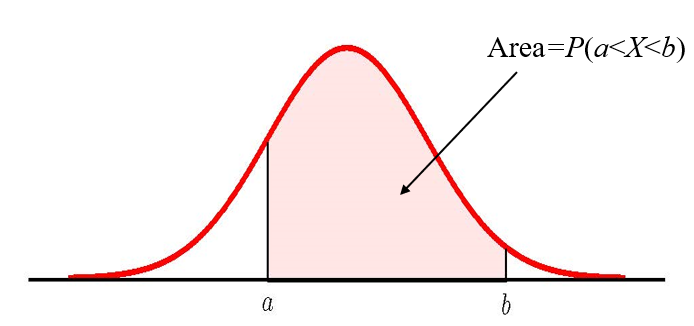
Probabilities for a normal random variable [latex]X[/latex] equal the area under the corresponding normal distribution curve. The probability that the value for [latex]X[/latex] falls in between the values [latex]x=a[/latex] and [latex]x=b[/latex] is the area under the normal distribution curve to the right of [latex]x=a[/latex] and to the left of [latex]x=b[/latex].
CALCULATING NORMAL PROBABILITIES IN EXCEL
To calculate probabilities associated with normal random variables in Excel, use the norm.dist(x,[latex]\mu[/latex],[latex]\sigma[/latex],logic operator) function.
- For x, enter the value for x.
- For [latex]\mu[/latex], enter the mean of the normal distribution.
- For [latex]\sigma[/latex], enter the standard deviation of the normal distribution.
- For the logic operator, enter true. Note: Because we are calculating the area under the curve, we always enter true for the logic operator.
The output from the norm.dist function is the probability that [latex]X \lt x[/latex]. That is, the output from the norm.dist function is the area to the left of value of x.
Visit the Microsoft page for more information about the norm.dist function.
NOTE
The norm.dist function always tells us the area to the left of the value entered for x.
- To find the area to the right of the value of x, we use 1-norm.dist(x,[latex]\mu[/latex],[latex]\sigma[/latex],true). This corresponds to the probability that [latex]X \gt x[/latex].
- To find the area in between x1 and x2 with [latex]x_1 \lt x_2[/latex], we use norm.dist(x2,[latex]\mu[/latex],[latex]\sigma[/latex],true)-norm.dist(x1,[latex]\mu[/latex],[latex]\sigma[/latex],true). This corresponds to the probability that [latex]x_1 \lt X \lt x_2[/latex].
An alternative approach in Excel is to use the norm.s.dist(z,true) function. In the norm.s.dist function, we enter the z-score for the corresponding value of x and the output will be the area to the left x.
CALCULATING [latex]\textcolor{white}x[/latex]-VALUES FOR A NORMAL DISTRIBUTION IN EXCEL
Given the area to the left of an (unknown) x-value, use the norm.inv(probability,[latex]\mu[/latex],[latex]\sigma[/latex]) function.
- For probability, enter the area to the left of x.
- For [latex]\mu[/latex], enter the mean of the normal distribution.
- For [latex]\sigma[/latex], enter the standard deviation of the normal distribution.
The output from the norm.inv function is the value of x so that the area to left of x equals the given probability. That is, the output from the norm.inv function is the value of x so that the [latex]P(X \lt x)=\mbox{probability}[/latex].
Visit the Microsoft page for more information about the norm.inv function.
NOTE
The norm.inv function requires that we enter the area to the left of the unknown x-value. If we are given the area to the right of the unknown x-value, we enter 1-area to the right for the probability in the norm.inv function. That is, given the area to the right of the x-value, we use norm.inv(1-area,[latex]\mu[/latex],[latex]\sigma[/latex]).
EXAMPLE
The final exam scores in a statistics class are normally distributed with a mean of 63 and a standard deviation of 5.
- Find the probability that a randomly selected student scored more than 65 on the exam.
- Find the probability that a randomly selected student scored less than 75.
- 90% of the students scored less than what value?
- 30% of the students scored more than what value?
Solution:
Let [latex]X[/latex] be the scores on the final exam.
- We want to find [latex]P(X \gt 65)[/latex]:
Function 1-norm.dist Answer Field 1 65 0.3446 Field 2 63 Field 3 5 Field 4 true The probability that a student scores more than 65 is 0.3446 (or 34.46%)

- We want to find [latex]P(X \lt 75)[/latex]:
Function norm.dist Answer Field 1 75 0.9918 Field 2 63 Field 3 5 Field 4 true The probability that a student scores less than 75 is 0.9918 (or 99.18%).
- We want to find the value of [latex]x[/latex] so that the area to the left of [latex]x[/latex] is 0.9.
Function norm.inv Answer Field 1 0.9 69.41 Field 2 63 Field 3 5 90% of the students scored below 69.41 points on the exam.
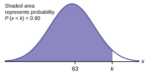
The 90th percentile is 69.4. This means that 90% of the test scores fall at or below 69.4 and 10% fall at or above. - We want to find the value of [latex]x[/latex] so that the area to the right of [latex]x[/latex] is 0.3. This is the same as finding the value of [latex]x[/latex] so that the area to left of [latex]x[/latex] is 0.7 (1-0.3).
Function norm.inv Answer Field 1 0.7 65.62 Field 2 63 Field 3 5 30% of the students scored more 65.62 points on the exam.
TRY IT
The golf scores for a school team are normally distributed with a mean of 68 and a standard deviation of 3.
- Find the probability that a randomly selected golfer scored less than 65.
- Find the probability that a randomly selected golfer scored more than 72.
Click to see Solution
-
Function norm.dist Answer Field 1 65 0.1587 Field 2 68 Field 3 3 Field 4 true -
Function 1-norm.dist Answer Field 1 72 0.0912 Field 2 68 Field 3 3 Field 4 true
EXAMPLE
A personal computer is used for office work at home, research, communication, personal finances, education, entertainment, social networking, and a myriad of other things. Suppose that the average number of hours a household personal computer is used for entertainment is 2 hours per day. Assume the times for entertainment are normally distributed and the standard deviation for the times is 0.5 hour.
- Find the probability that a household personal computer is used for entertainment between 1.8 and 2.75 hours per day.
- Find the maximum number of hours per day that the bottom quartile of households uses a personal computer for entertainment.
Solution:
Let [latex]X[/latex] be the amount of time (in hours) a household personal computer is used for entertainment.
- We want to find [latex]P(1.8 \lt X \lt 2.75)[/latex].
Function norm.dist -norm.dist Answer Field 1 2.75 1.8 0.5886 Field 2 2 2 Field 3 0.5 0.5 Field 4 true true The probability a household computer is used for entertainment between 1.8 and 2.75 hours a day is 0.5886 (or 58.86%).

- We need to find the value x so that 25% of the number of hours as less than this value.
Function norm.inv Answer Field 1 0.25 1.66 Field 2 2 Field 3 0.5 25% of the value are less than 1.66 hours.

TRY IT
The golf scores for a school team are normally distributed with a mean of 68 and a standard deviation of 3. Find the probability that a golfer scored between 66 and 70.
Click to see Solution
| Function | norm.dist | -norm.dist | Answer |
| Field 1 | 70 | 66 | 0.4950 |
| Field 2 | 68 | 68 | |
| Field 3 | 3 | 3 | |
| Field 4 | true | true |
EXAMPLE
There are approximately one billion smartphone users in the world today. In the United States the ages of smartphone users from 13 to 55+ follow a normal distribution with approximate mean and standard deviation of 36.9 years and 13.9 years, respectively.
- Determine the probability that a random smartphone user in the age range 13 to 55+ is between 23 and 64.7 years old.
- Determine the probability that a randomly selected smartphone user in the age range 13 to 55+ is at most 50.8 years old.
- 80% of the users in the age range 13 to 55+ are less than what age?
- 40% of the ages that range from 13 to 55+ are at least what age?
Solution:
-
Function norm.dist -norm.dist Answer Field 1 64.7 23 0.8186 Field 2 36.9 36.9 Field 3 13.9 13.9 Field 4 true true The probability a smartphone user is between 23 and 64.7 years of age is 0.8186 (or 81.86%).
-
Function norm.dist Answer Field 1 50.8 0.8413 Field 2 36.9 Field 3 13.9 Field 4 true The probability that a smartphone user is less than 50.8 years of age is 0.8413 (or 84.13%).
-
Function norm.inv Answer Field 1 0.8 48.6 Field 2 36.9 Field 3 13.9 80% of the smartphone users in the age range 13 – 55+ are 48.6 years old or less.
-
Function norm.inv Answer Field 1 0.6 40.42 Field 2 36.9 Field 3 13.9 40% of the smartphone users in the age range 13 – 55+ are older than 40.42 years of age.
TRY IT
There are approximately one billion smartphone users in the world today. In the United States the ages of smartphone users from 13 to 55+ follow a normal distribution with approximate mean and standard deviation of 36.9 years and 13.9 years, respectively.
- 30% of smartphone users are older than what age?
- What is the probability that the age of a randomly selected smartphone user in the range 13 to 55+ is less than 27 years old.
Click to see Solution
-
Function norm.inv Answer Field 1 0.7 44.19 Field 2 36.9 Field 3 13.9 -
Function norm.dist Answer Field 1 27 0.2382 Field 2 36.9 Field 3 13.9 Field 4 true
EXAMPLE
A citrus farmer who grows mandarin oranges finds that the diameters of mandarin oranges harvested on his farm follow a normal distribution with a mean diameter of 5.85 cm and a standard deviation of 0.24 cm.
- Find the probability that a randomly selected mandarin orange from this farm has a diameter larger than 6.0 cm.
- 90% of the diameters of the mandarin oranges are less than what value?
- 35% of the diameters of the mandarin oranges are greater than what value?
Solution:
-
Function 1-norm.dist Answer Field 1 6 0.2660 Field 2 5.85 Field 3 0.24 Field 4 true The probability an orange has a diameter greater than 6 cm is 0.2660 (or 26.60%).
-
Function norm.inv Answer Field 1 0.9 6.16 Field 2 5.85 Field 3 0.24 90% of the diameters of the oranges are less than 6.16 cm.
-
Function norm.inv Answer Field 1 0.65 5.94 Field 2 5.85 Field 3 0.24 35% of the diameters of the oranges are greater than 5.94 cm.
Watch this video: Excel 2013 Statistical Analysis #39: Probabilities for Normal (Bell) Probability Distribution by ExcelIsFun [24:07]
Concept Review
The normal distribution, which is continuous, is the most important of all the probability distributions. Its graph is bell-shaped. This bell-shaped curve is used in almost all disciplines. The probability that the value for a normal random variable falls in between the values [latex]x=a[/latex] and [latex]x=b[/latex] is the area under the normal distribution curve to the right of [latex]x=a[/latex] and to the left of [latex]x=b[/latex].
Attribution
“6.2 Using the Normal Distribution“ in Introductory Statistics by OpenStax is licensed under a Creative Commons Attribution 4.0 International License.
