4.9 – Theory of Labour Markets
Learning Objectives
- Describe the demand for labour in perfectly competitive output markets
- Describe the demand for labour in imperfectly competitive output markets
- Identify what determines the going market rate
Clear It Up
What is the labour market?
The labour market, like all markets, has a demand and a supply. Why do firms demand labour? Why is an employer willing to pay you for your labour? It’s not because the employer likes you or is socially conscious. Rather, it’s because your labour is worth something to the employer--your work brings in revenues to the firm. How much is an employer willing to pay? That depends on the skills and experience you bring to the firm.
If a firm wants to maximize profits, it will never pay more (in terms of wages and benefits) for a worker than the value of his or her marginal productivity to the firm. We call this the first rule of labour markets.
Suppose a worker can produce two widgets per hour and the firm can sell each widget for $4 each. Then the worker is generating $8 per hour in revenues to the firm, and a profit-maximizing employer will pay the worker up to, but no more than, $8 per hour, because that is what the worker is worth to the firm.
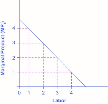
Recall the definition of marginal product. Marginal product is the additional output a firm can produce by adding one more worker to the production process. Since employers often hire labour by the hour, we’ll define marginal product as the additional output the firm produces by adding one more worker hour to the production process. In this chapter, we assume that workers are homogeneous—they have the same background, experience and skills and they put in the same amount of effort. Thus, marginal product depends on the capital and technology with which workers have to work.
A typist can type more pages per hour with an electric typewriter than a manual typewriter, and he or she can type even more pages per hour with a personal computer and word processing software. A ditch digger can dig more cubic feet of dirt in an hour with a backhoe than with at shovel.
Thus, we can define the demand for labour as the marginal product of labour times the value of that output to the firm.
| # Workers (L) | 1 | 2 | 3 | 4 |
|---|---|---|---|---|
| MPL | 4 | 3 | 2 | 1 |
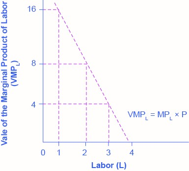
On what does the value of each worker’s marginal product depend? If we assume that the employer sells its output in a perfectly competitive market, the value of each worker’s output will be the market price of the product. Thus,
Demand for Labour = MPL x P = Value of the Marginal Product of Labour
[latex]{\scriptsize \begin{equation} \text{The Demand for Labour} = \text{MP}_{\text{L}} \times \text{P} = \text{Value of the Marginal Revenue Product} \end{equation}\scriptsize}[/latex]
We show this in Table 4.9b, which is an expanded version of Table 4.9a.
| # Workers (L) | 1 | 2 | 3 | 4 |
|---|---|---|---|---|
| MPL | 4 | 3 | 2 | 1 |
| Price of Output | $4 | $4 | $4 | $4 |
| VMPL | $16 | $12 | $8 | $4 |
Note that the value of each additional worker is less than the ones who came before.
Demand for Labour in Perfectly Competitive Output Markets
The question for any firm is how much labour to hire.
We can define a Perfectly Competitive Labour Market as one where firms can hire all the labour they wish at the going market wage. Think about secretaries in a large city. Employers who need secretaries can probably hire as many as they need if they pay the going wage rate.
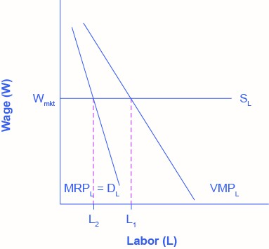
Graphically, this means that firms face a horizontal supply curve for labour.
Given the market wage, profit maximizing firms hire workers up to the point where: [latex]{\scriptsize \begin{equation} \text{W}_{\text{mkt}} = \text{VMP}_{\text{L}}\end{equation}\scriptsize}[/latex]
In a perfectly competitive labour market, firms can hire all the labour they want at the going market wage. Therefore, they hire workers up to the point L1 where the going market wage equals the value of the marginal product of labour.
Clear It Up
Derived Demand
Economists describe the demand for inputs like labour as a derived demand. Since the demand for labour is MPL*P, it is dependent on the demand for the product the firm is producing. We show this by the P term in the demand for labour. An increase in demand for the firm’s product drives up the product’s price, which increases the firm’s demand for labour. Thus, we derive the demand for labour from the demand for the firm’s output.
Demand for Labour in Imperfectly Competitive Output Markets
If the employer does not sell its output in a perfectly competitive industry, they face a downward sloping demand curve for output, which means that in order to sell additional output the firm must lower its price. This is true if the firm is a monopoly, but it’s also true if the firm is an oligopoly or monopolistically competitive. In this situation, the value of a worker’s marginal product is the marginal revenue, not the price. Thus, the demand for labour is the marginal product times the marginal revenue.
[latex]{\scriptsize \begin{equation} \text{The Demand for Labour} = \text{MP}_{\text{L}} \times \text{MR} = \text{Marginal Revenue Product} \end{equation}\scriptsize}[/latex]
| # Workers (L) | 1 | 2 | 3 | 4 |
|---|---|---|---|---|
| MPL | 4 | 3 | 2 | 1 |
| Marginal Revenue | $4 | $3 | $2 | $1 |
| MRPL | $16 | $9 | $4 | $1 |
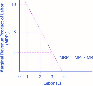
Everything else remains the same as we described above in the discussion of the labour demand in perfectly competitive labour markets. Given the market wage, profit-maximizing firms will hire workers up to the point where the market wage equals the marginal revenue product, as Figure 4.9d shows.
Clear It Up
The probabilities assigned to events by a distribution function on a sample space are given by.
Do Profit Maximizing Employers Exploit Labour?
Every other worker brings in more revenue than the firm pays him or her. This has sometimes led to the claim that employers exploit workers because they do not pay workers what they are worth. Let’s think about this claim. The first worker is worth $x to the firm, and the second worker is worth $y, but why are they worth that much? It is because of the capital and technology with which they work. The difference between workers’ worth and their compensation goes to pay for the capital, technology, without which the workers wouldn’t have a job. The difference also goes to the employer’s profit, without which the firm would close and workers wouldn’t have a job. The firm may be earning excessive profits, but that is a different topic of discussion.
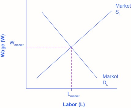
What Determines the Going Market Wage Rate?
The labour market has demand and supply curves like other markets. The demand for labour curve is a downward sloping function of the wage rate. The market demand for labour is the horizontal sum of all firms’ demands for labour. The supply for labour curve is an upward sloping function of the wage rate. This is because if wages for a particular type of labour increase in a particular labour market, people with appropriate skills may change jobs, and vacancies will attract people from outside the geographic area. The market supply for labour is the horizontal summation of all individuals’ supplies of labour.
Like all equilibrium prices, the market wage rate is determined through the interaction of supply and demand in the labour market. Thus, we can see for competitive markets the wage rate and number of workers hired. Figure by Steven A. Greenlaw & David Shapiro (OpenStax), licensed under CC BY 4.0.
The FRED database has a great deal of data on labour markets, starting at the wage rate and number of workers hired [New Tab].
The United States Census Bureau for the Bureau of Labor Statistics publishes The Current Population Survey, which is a monthly survey of households (link is on that page), which provides data on labour supply, including numerous measures of the labour force size (disaggregated by age, gender and educational attainment), labour force participation rates for different demographic groups, and employment. It also includes more than 3,500 measures of earnings by different demographic groups.
The Current Employment Statistics, which is a survey of businesses, offers alternative estimates of employment across all sectors of the economy.
The link labeled "Productivity and Costs" has a wide range of data on productivity, labour costs and profits across the business sector.
Attribution
Except where otherwise noted, this chapter is adapted from "Theory of Labor Markets" In Microeconomics (OpenStax) (LibreText) by OpenStax, licensed under CC BY 4.0. A derivative of Principles of Microeconomics (OpenStax) by Steven A. Greenlaw & Timothy Taylor, licensed under CC BY 4.0.
Access for free at Principles of Microeconomics
Media Attributions
- Figure © Steven A. Greenlaw & David Shapiro (OpenStax) is licensed under a CC BY (Attribution) license
- Figure © Steven A. Greenlaw & David Shapiro (OpenStax) is licensed under a CC BY (Attribution) license
- Figure © Steven A. Greenlaw & David Shapiro (OpenStax) is licensed under a CC BY (Attribution) license
- Figure © Steven A. Greenlaw & David Shapiro (OpenStax) is licensed under a CC BY (Attribution) license
- Figure © Steven A. Greenlaw & David Shapiro (OpenStax) is licensed under a CC BY (Attribution) license
