4.7 – The Demand for Labour
Learning Objectives
- Explain and graph the demand for labour in perfectly competitive output markets
- Explain and graph the demand for labour in imperfectly competitive output markets
- Demonstrate how supply and demand interact to determine the market wage rate
Demand for Labour in Perfectly Competitive Output Markets
The question for any firm is how much labour to hire.
We can define a perfectly competitive labour market as one where firms can hire all the labour they wish at the going market wage. Think about secretaries in a large city. Employers who need secretaries can probably hire as many as they need if they pay the going wage rate.
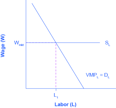
Graphically, this means that firms face a horizontal supply curve for labour, as seen in Figure 4.7a Equilibrium Employment for Firms in a Competitive Labour Market.
Given the market wage, profit maximizing firms hire workers up to the point where: [latex]{\scriptsize \begin{equation} \text{W}_{\text{mkt}} = \text{VMP}_{\text{L}}\end{equation}\scriptsize}[/latex]

Figure 4.7a Equilibrium Employment for Firms in a Competitive Labour Market (Text Version)
The graph shows the Marginal Product of Labour. The x-axis is Labour. The y-axis is Wage. The curve proceeds from right to left in a downward direction. A horizontal line (SL) indicating the going market wage projects from about halfway up the y-axis at point Wmkt. Where the curve and the horizontal line meet, it is point L1. [latex]{\scriptsize \begin{equation} \text{W}_{\text{mkt}} = \text{VMP}_{\text{L}}\end{equation}\scriptsize}[/latex]
Derived Demand
Economists describe the demand for inputs like labour as a derived demand. Since the demand for labour is MPL*P, it is dependent on the demand for the product the firm is producing. We show this by the P term in the demand for labour. An increase in demand for the firm’s product drives up the product’s price, which increases the firm’s demand for labour. Thus, we derive the demand for labour from the demand for the firm’s output.
Try It
Try It (Text version)
H5P Figure (Text Version)
The graph shows the Marginal Product of Labour. The x-axis is Labour. The y-axis is Wage. The curve proceeds from right to left in a downward direction. A horizontal line (SL) indicating the going market wage projects from about halfway up the y-axis at point Wmkt. Where the curve and the horizontal line meet, it is point L1. [latex]{\scriptsize \begin{equation} \text{VMP}_{\text{L}} = \text{D}_{\text{L}}\end{equation}\scriptsize}[/latex].
- Considering the figure above, the demand for labour is considered a(n) ________.
- Perfect competitive labour market
- Derived demand labour market
- Imperfectly competitive labour market
Check your Answers: [1]
Activity source: “The Demand for Labor” In by Lumen Learning, licensed under CC BY. / Converted to H5P and Text.
Demand for Labour in Imperfectly Competitive Output Markets
| # Workers (L) | 1 | 2 | 3 | 4 |
|---|---|---|---|---|
| MPL | 4 | 3 | 2 | 1 |
| Marginal Revenue | $4 | $3 | $2 | $1 |
| MRPL | $16 | $9 | $4 | $1 |
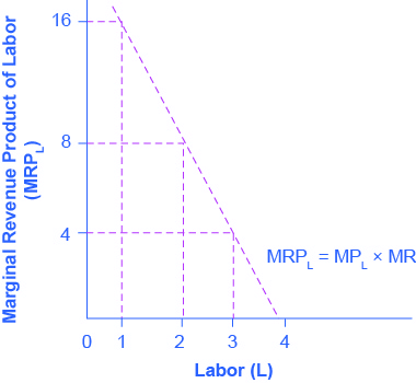
Everything else remains the same as we described above in the discussion of the labour demand in perfectly competitive labour markets. Given the market wage, profit-maximizing firms will hire workers up to the point where the market wage equals the marginal revenue product, as Figure 3 shows.
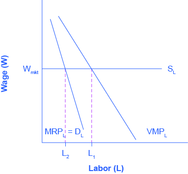
Figure 4.7c Equilibrium Level of Employment for Firms with Market Power
The graph shows the Marginal Product of Labour. The x-axis is Labour. The y-axis is Wage. A horizontal line indicating the going market wage projects from about halfway up the y-axis. Two curves are included in order to demonstrate the difference for firms with market power. The first curve represents normal firms, and proceeds from right to left in a downward direction; where it intersects the Wage horizontal line, it is point L1. The second curve, representing firms with market power, is steeper, and intersects the Wage line earlier (at a lower level of employment), at point L2, where the going market wage equal’s the firm’s marginal revenue product.
Do profit maximizing employers exploit labour?
If you look back at Figure 14.6 Equilibrium Level of Employment for Firms with Market Power, you will see that the firm only pays the last worker it hires what they’re worth to the firm. Every other worker brings in more revenue than the firm pays him or her. This has sometimes led to the claim that employers exploit workers because they do not pay workers what they are worth. Let’s think about this claim. The first worker is worth $x to the firm, and the second worker is worth $y, but why are they worth that much? It is because of the capital and technology with which they work. The difference between workers’ worth and their compensation goes to pay for the capital, and other inputs in the production process. The difference also goes to the employer’s profit, without which the firm would close and workers wouldn’t have a job. The firm may be earning excessive profits, but that is a different topic of discussion.
Try It
Try It (Text version)

H5P Figure (Text Version)
The graph shows the Marginal Product of Labour. The x-axis is Labour. The y-axis is Wage. A horizontal line indicating the going market wage projects from about halfway up the y-axis. Two curves are included in order to demonstrate the difference for firms with market power. The first curve represents normal firms, and proceeds from right to left in a downward direction; where it intersects the Wage horizontal line, it is point L1. The second curve, representing firms with market power, is steeper, and intersects the Wage line earlier (at a lower level of employment), at point L2, where the going market wage equal’s the firm’s marginal revenue product.
- Considering the graph above, the demand for labour is considered a(n) ________.
- Imperfectly competitive labour market
- Perfect competitive labour market
- Derived demand labour market
Check your Answers: [2]
Activity source: “The Demand for Labor” In by Lumen Learning, licensed under CC BY. / Converted to H5P and Text.
What Determines the Going Market Wage Rate?
We learned earlier that the labour market has demand and supply curves like other markets. The demand for labour curve is a downward sloping function of the wage rate. The market demand for labour is the horizontal sum of all firms’ demands for labour. The supply for labour curve is an upward sloping function of the wage rate. This is because if wages for a particular type of labour increase in a particular labour market, people with appropriate skills may change jobs, and vacancies will attract people from outside the geographic area. The market supply for labour is the horizontal summation of all individuals’ supplies of labour.
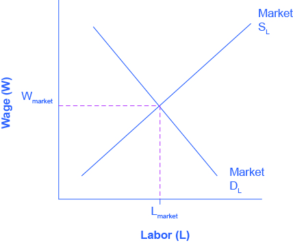
Like all equilibrium prices, the market wage rate is determined through the interaction of supply and demand in the labor market. Thus, we can see in Figure 4, the wage rate and number of workers hired in a competitive labor market.
Watch it!
Watch this video for a nice overview of the labour market, and the ways that supply and demand interact to determine wages. The video will also introduce some of the key concepts we’ll discuss soon, including monopsonies, unions, discrimination, and minimum wage laws.
Watch Labor markets and minimum wage: Crash Course economics #28 (11 mins) on YouTube
Video Source: CrashCourse. (2016, March 27). Labor markets and minimum wage: Crash Course economics #28 [Video]. YouTube. https://youtu.be/mWwXmH-n5Bo
Try It
Try It (Text version)
- Supply and demand determine the labour market at equilibrium. ________ supply the labour while ________ demand the labour. Fill in the two blanks with the appropriate terms:
- Workers; firms
- Firms; workers
- Workers; consumers
Check your Answers: [3]
Activity source: “The Demand for Labor” In by Lumen Learning, licensed under CC BY. / Converted to H5P and Text.
Additional Key Terms
collective bargaining:
negotiations between unions and a firm or firms
labour union:
an organization of workers that negotiates with employers over wages and working conditions
perfectly competitive labour market:
a labour market where neither suppliers of labour nor demanders of labour have any market power; thus, an employer can hire all the workers they would like at the going market wage
marginal revenue product of labour:
the marginal product of an additional worker multiplied by the marginal revenue to the firm of the additional worker’s output
Attribution
Except where otherwise noted, this chapter is adapted from “The Demand for Labor” In Microeconomics by Lumen Learning, licensed under CC BY 4.0. A derivative of “The Theory of Labor Markets” In Principles of Economics 2e by Steven A. Greenlaw & David Shapiro (OpenStax), licensed under CC BY 4.0.
Access for free at Principles of Economics 2e
Media Attributions
- Figure © Steven A. Greenlaw & David Shapiro (OpenStax) is licensed under a CC BY (Attribution) license
- Figure © Steven A. Greenlaw, & David Shapiro (openstax) is licensed under a CC BY (Attribution) license
- Figure © Steven A. Greenlaw & David Shapiro (OpenStax) is licensed under a CC BY (Attribution) license
- Figure © Steven A. Greenlaw & David Shapiro (OpenStax) is licensed under a CC BY (Attribution) license
- Figure © Steven A. Greenlaw, & David Shapiro (openstax) is licensed under a CC BY (Attribution) license
- Figure © Steven A. Greenlaw & David Shapiro (OpenStax) is licensed under a CC BY (Attribution) license
- 1. a) Correct. In a perfectly competitive labour market, firm can hire all the labour they want at the going market wage. Therefore, they hire workers up to the point L1 where the going market wage equals the value of the marginal product of labour. ↵
- Question 1) a) Correct. In a imperfectly competitive labour market, they choose the number of workers,(L2) where the going market wage equals the firm's marginal revenue product. Note that since marginal revenue is less than price, the demand for labour for a firm which has market power in its output market is less than the demand for labour(L1) for a perfectly competitive firm. As a result, employment will be lower in an imperfectly competitive industry than in a perfectly competitive industry. ↵
- 1. a) Correct. In a competitive labour market, the equilibrium wage and employment level are determined where the market demand for labour equals the market supply of labour. ↵
