
We’ve learned that, by using today’s age-specific mortality rates, we can compute expected life years remaining for people of any age alive today. This is only a projection based on the assumption that mortality rates will not change in the future.
We also saw that survival probabilities from birth to any age x can be read off the Life Table. Similarly, survival probabilities from any age x to any other age x+t can be derived by dividing the number of people entering age x+t by the number of people who entered age x.
Let’s squeeze a little more juice out of the Life Table and see what it can tell us about the age distribution of the population.

If the same number of newborns are born each year, and if mortality rates do not change – that is, if the population is what we call “stationary” – then the “l” column of the Life Table will give us the population’s breakdown by age, scaled up or down depending on whether the number of newborns used in the Life Table is higher or lower than the actual number of newborns. If there literally are 100,000 newborns every year, and 99% make it to age 1, and 98% make it to age 5, then every year there will be 100,000 newborns, 99,000 one-year olds, 98,000 five year olds etc.
If the population were not stationary, but stable, with the number of newborns growing or shrinking at some constant rate r each year, then again we could determine the population by age by looking at the “l” column of the Life Table, but we would have to perform a small adjustment. If the population were growing in a stable way, so that each successive cohort of newborns was r percent larger than the previous cohort, and letting x be actual ages, not age groups, we would have to multiply each lx by e-x (e for exponential, not life expectancy!) to show that the older groups come from smaller generations of newborns. If the population were stably shrinking, we would multiply each lx by ex to show that the older groups come from larger generations of newborns. Once we had performed this adjustment, the age distribution of the Life Table would be the same as the age distribution of the population.

As we get older, we normally have fewer life years remaining. But when mortality is very high in a particular age group, those who survive to the next age group may have a higher expected number of life years remaining than before! For example, in 2009, the expectation of life years remaining for newborns (both sexes together) in Afghanistan was 48.3, but the expectation of life years remaining for 1 year-olds was 54.7, and for 5 year-olds, 55.[1] Because of high infant mortality, a Paradox of the Life Table can be expected in places of great poverty.
What is going on? Recall that expected life years remaining at age x is equal to:
ex = Tx divided by lx.
As we get older, we run out of life and T falls, so the numerator falls and our life years remaining fall.
However, the denominator is also getting smaller as we get older. The number of people our age, our birth cohort, is shrinking. If, because of a pandemic, for example, the number of people our age is shrinking faster than the life years our group can expect to enjoy is shrinking, expected life years remaining for the average person in our age group could be higher after the pandemic.
The survivors of the pandemic would have more life years left to live than what the average person in our age group had before the pandemic began. This concept will be relevant to understanding the Black-White Crossover Effect to be described in Chapter 9.


If you do more reading in demography, you will soon come across so-called model Life Tables. Model Life Tables are stylized Life Tables, each of which attempts to generalize the mortality data of a group of similar nations. “Similar” nations experience similar climate, have similar lifestyles, are at a similar stage of economic development, and have access to similar medical care.
Model Life Tables are constructed by using the data from a related group of countries to correlate the probability of dying in one age group to the probability of dying in the next age group and thus generate a set of typical age-specific mortality rates.
Using model Life Tables, a nation can compare its mortality data with those of similar nations.
Also, if you don’t have all the age-specific mortality rates to make a Life Table for your nation, you could use one of these model Life Tables to fill in the gaps in this way:
1) Choose which model Life Table to use based on your population’s level of economic development, and how its fertility and mortality rates compare. There are different model Life Tables for different kinds of countries.
2) Compare some representative datum from your nation e.g. life expectancy at birth, age-specific mortality rate for 20-25 year old males etc. to the corresponding datum in the model Life Table.
3) Scale the model Life Table up or down until the two data points match.
4) Read the data you are interested in off the scaled model Life Table.
Instead of working with existing model Life Tables (which rapidly become outdated), today’s scholar equipped with statistical training and computers would be likely be forming their own estimates of any missing data. They would correlate any age-specific mortality rate data that they do have to past values, to the values of other age groups’ mortality rates, and to socioeconomic indicators and come up with a way to guess the missing numbers.
In our next chapter we will see that scholars used this kind of statistical work to predict what Puerto Rico’s mortality rates would have been had Hurricane Maria not occurred.
For more information on model Life Tables, see C.J.L. Murray et al. in the References.

We noticed previously that male mortality rates tend to be higher than female mortality rates. There are “extra” male deaths in that sense. But that doesn’t mean there is any foul play. To check whether there is anything suspicious going on, we should compare male mortality relative to female mortality in our nation to the male mortality relative to female mortality in similar nations, i.e. using model Life Tables.
Looking at Table 7-2, we see that male mortality rates during 2010-2013 were very different for the average Canadian compared to First Nations people with Indian Status. Neither set of mortality rates can be used as a model for the other. Something seems wrong.
We also observe that male mortality for Status men was not as much higher compared to Status women as the mortality of Canadian men compared to Canadian women. This was not because of an advantage that Status men had; sadly, it was because Status women’s mortality was significantly higher than the mortality of the average Canadian woman.

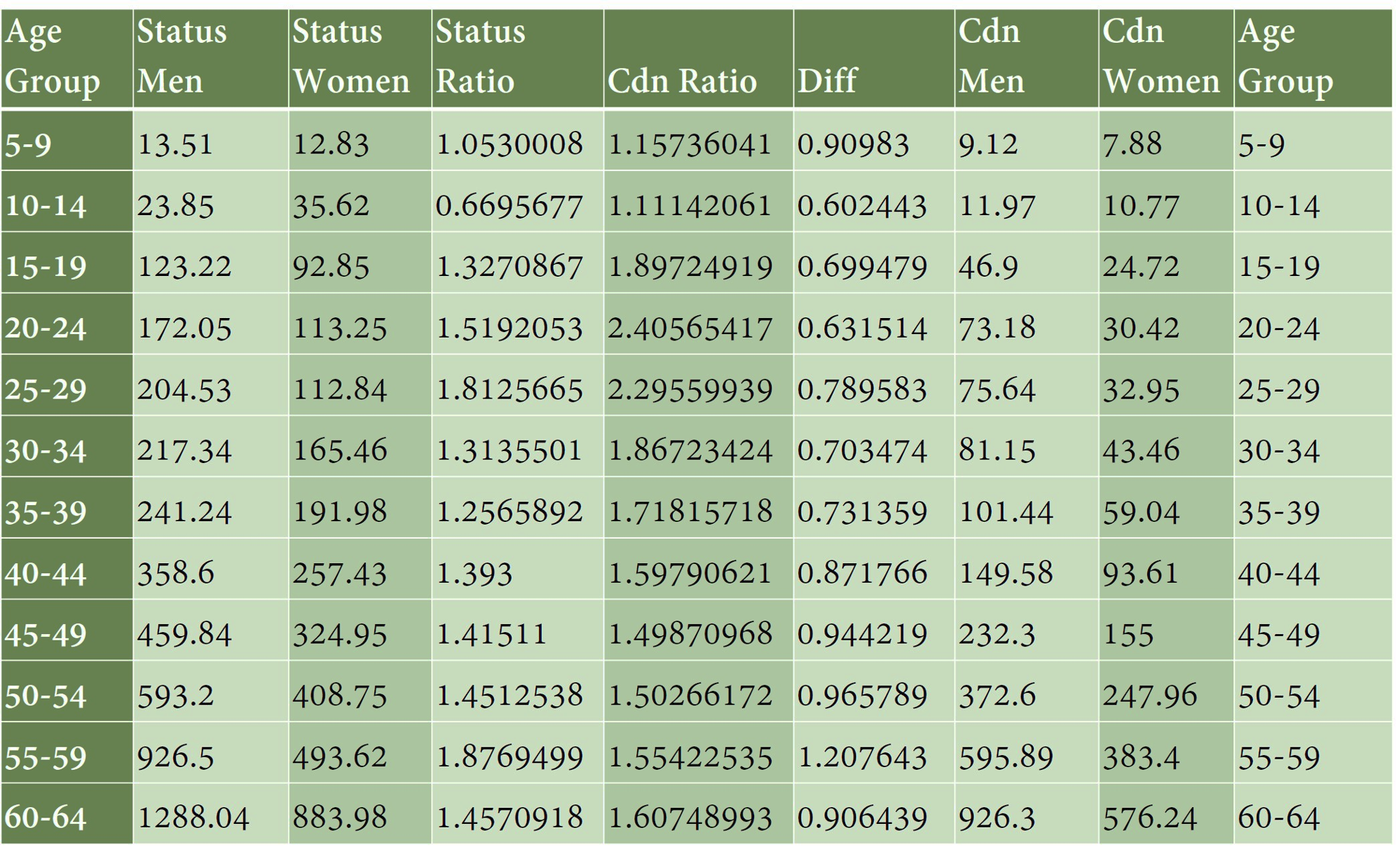
Akee and Feir (2016, 2018) found that, between 2010 and 2013, women with Indian Status ages 5-64 had mortality rates 3-5 times higher than those of the average Canadian woman ages 5-64. Status men had mortality rates 2-4 times higher than Canadian men. These are very distressing facts, but keep in mind that mortality rates for Canadian men and women are very very low to begin with.
Akee and Feir (2016) write, “Our estimate of excess mortality for Status women and girls is almost three times the number of all missing and murdered Indigenous women and girls reported by the RCMP.” They noted that most of the extra deaths were due to non-violent causes. Chronic living conditions, especially poverty, were important in explaining the higher mortality.

Figuring out how many extra deaths were experienced by Status women is not as easy as it looks. You might think that we could just apply the “normal” mortality rates for Canadian females to the number of Status women of any age to get the expected number of deaths under normal circumstances, and then compute how many more deaths were actually experienced by Status women. But the number of Status women of any age is too small already compared to what it should be, because of high mortality. We need to know what happened to the cohort of women from the time they were born. Unfortunately, birth information for Status persons is not well organized.
In Canada and elsewhere, much work remains to be done in order to understand, honour and enhance Indigenous peoples’ lived experience.

Jiang, Feldman, and Jin (2005)[2] also wanted to find the number of missing women, in their case women living in China, and they had similar data problems. They didn’t know how many women should have been born, or how many should have been entering each age group. They mistrusted the government’s records as to how many girls had been born. They even mistrusted the female mortality data. But they had one advantage: they had accurate and unsuspicious birth records for males.
The team began by assuming a sex ratio at birth of 1.06 due to China being in a more northerly climate (the sex ratio is slightly lower in southern climates); for each generation of children born in the same year, i.e. each cohort, they began with 106 infant boys in the numerator and 100 infant girls in the denominator as the expected sex ratio at birth.
To get the sex ratio at any age x, they first multiplied the numerator (the 106 infant boys) by the survival probability from birth to age x. They used a Chinese Life Table to find the survival probability. This gave them the expected number of boys age x. They then multiplied the denominator (the 100 infant girls) by a model Life Table’s survival probability for girls from birth to age x. This gave them the expected number of girls age x.
Dividing the numerator by the denominator, they obtained the expected sex ratio for age x.
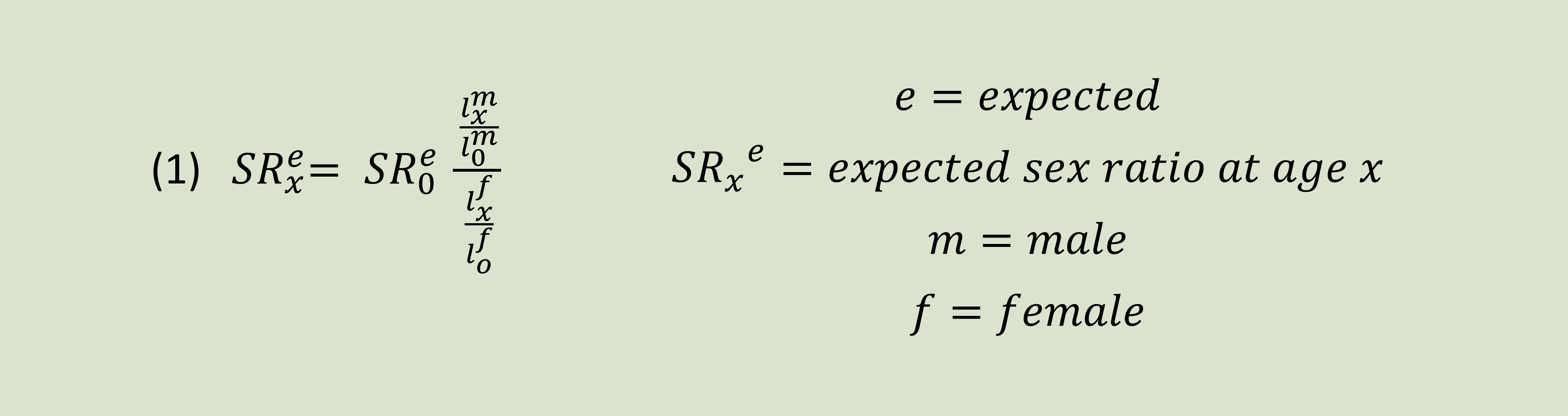
The ![]() is the probability of men surviving from birth (age 0) to age x, as read off the Life Table.
is the probability of men surviving from birth (age 0) to age x, as read off the Life Table.
The ![]() is the probability of women surviving from birth to age x, as read off the model Life Table.
is the probability of women surviving from birth to age x, as read off the model Life Table.
Next, Li et. al went looking for census and other estimates of what the actual number of boys age x had been x years after the cohort in question was born. They divided the actual number of boys by the expected sex ratio to find what the number of girls age x should have been.
 They compared this expected number of girls age x to the actual number of girls age x recorded in the census or other estimates for that year.
As a result of their calculations, the team estimated that 35 million Chinese females were lost over the course of the twentieth century. That would be about 4.65 percent of all females who were otherwise expected to be born and survive.
What possibly happened to these girls and women? Think of the three drivers of population change.
-
- Fertility: the actual sex ratio at birth was higher than 1.06 due to infanticide at the time of birth and the birth not being reported as a live birth, or, in the last part of the twentieth century, sex-specific abortion.
- Mortality: the actual mortality rates were higher than the model Life Table mortality rates: a greater fraction of girls and women died or were killed in China than in comparable countries.
- Migration: some women emigrated (at a higher rate than men their age) (unlikely) or were forcibly removed to another country (also unlikely).
The twentieth century was a very difficult century for China. It included a political revolution, a cultural revolution, three episodes of civil war, a famine, an invasion by the Japanese, and a period of strict birth control measures enforced by the government.
Despite these pressures, most girls and women were loved and cherished.
Discrimination against female children will be discussed more in Chapter 24. For now, we will talk more about mortality.

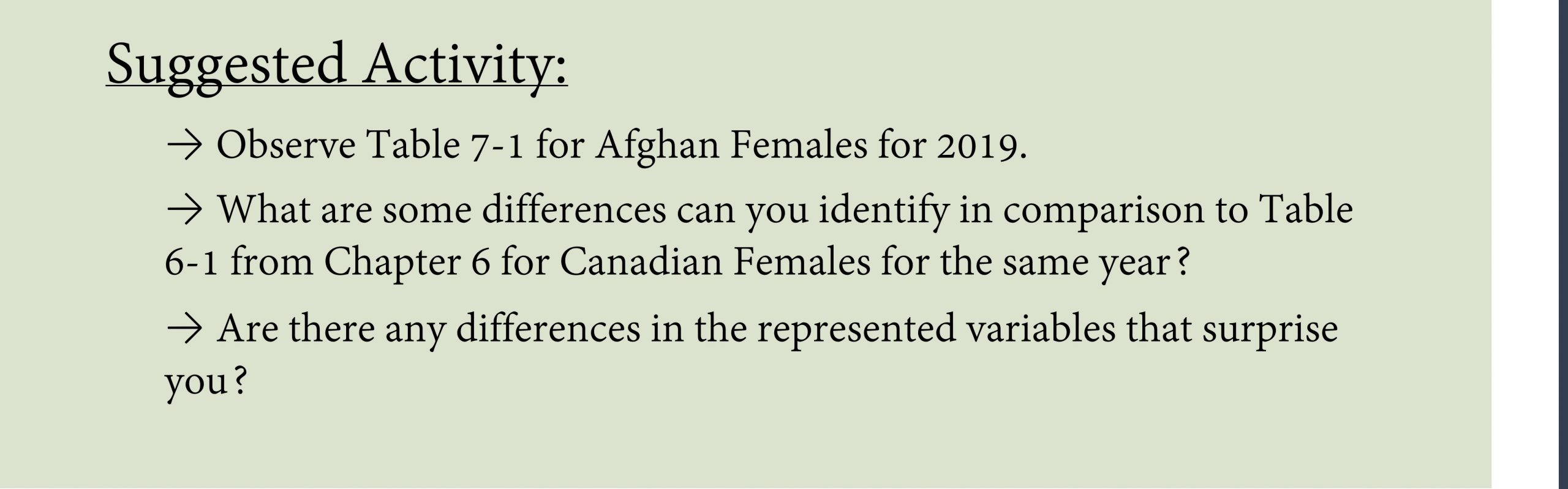
- Consider Table 7-1. What is the probability that an Afghan female born in 2019 will become at least 20 years old?
- According to the same Table, what is the probability that an Afghan female born in 2019, having just turned 1 year old, will become at least 20 years old?
- Compare your answers in 1. and 2. Is this a paradox? Where/ where else can you see the Paradox of the Life Table in Table 7-1?
- The natural sex ratio at birth for the nation of Alametra is 1.05. From 100,000 hypothetical new-born females, 98,500 are alive at age 25 in Alametra and similar countries in the region. In similar countries, from 100,000 hypothetical newborn males, 97,000 are alive at age 25. In Alametra today, there are 1.5 million women and 1.2 million men. How many men appear to be missing from Alametra? Why might these men be missing?
- In Country X, there are 28,275 females age 15 and 30,000 males age 15. Migration of children under 15 has been negligible. In a life table that uses mortality rates typical for countries at a similar state of economic and demographic transition, females have a 95 % chance of surviving until age 15, and males have a 94 % chance of surviving until age 15. The sex ratio at birth should be 1.05. For Country X, what is the number of missing females among those born 15 years ago?
see "stable population"
The Paradox of the Life Table occurs whenever an older age group has a greater number of expected life years remaining than does a younger age group.
The Black-White Crossover Effect is the phenomenon of Black people age x having more expected life years remaining than White people age x, for x>75 years of age
Model Life Tables are generalized Life Tables for a particular group of countries, based on their typical age-specific mortality rates.
Chronic living conditions are everyday living conditions, with the usual risks of dying.
