In demography we like to predict what the population will look like in the future. Since almost anything can happen to birth, death, and immigration rates, there is no way to know this for sure. We like to assume that “present trends continue.” We can do this by  studying a hypothetical “stable population” based on today’s fertility and mortality rates.

A stable population is one where:

• There is no immigration or emigration
•  age-specific fertility rates do not change
• age-and-sex-specific mortality rates do not change
• enough time has passed for the age structure of the population to stabilize.

Why does it take time for a population to stabilize?  Well, just because fertility rates stay the same this year and next doesn’t mean that the birth rate won’t change.  The birth rate depends not only on fertility rates but also on the number of women of childbearing age, which could be different next year than it is this year.

Similarly, as we learned when standardizing for age, death rates depend not only on age-specific mortality rates but also on the age distribution of the population.  So death rates won’t stabilize until the age structure stabilizes.

Consider a population where fertility has recently fallen. The birth rate will not necessarily immediately fall. Fertility may have dropped, but there may be a larger number of women of childbearing age this year than there was last year due to higher fertility rates in the past.

Between 2004 and 2009, Canada experienced a small baby boom. The crude birth rate rose from 10.5 births per 1000 to 11.3 per 1000.   Some of this baby boom was likely due to the fact that, during the late 1940s and the 1950s and the early 1960s, many Canadians were born – our Baby Boom Generation. The grandchildren of these boomers were reaching child-bearing age between 2004 and 2009. Also, many of the children of the baby boom generation had delayed having children and were having them at this time.

The birth rate and death rate are not going to stabilize until fertility rates and mortality rates have been constant for some time, long enough for the age structure to stabilize. Once the age structure stabilizes, birth and death rates can stabilize too, and the overall rate of population growth or shrinkage will stabilize.

Later in this chapter we will learn how to calculate the age structure of a stable population.  We will also learn how to calculate the rate of growth (or shrinkage) of a stable population.  The rate of growth of a stable population is called the intrinsic rate of natural increase.  It’s “natural” because it comes from the fertility and mortality of the population, and not because of immigration or emigration.   It’s “intrinsic” because it derives from the fertility and mortality rates and will eventually emerge no matter what the initial population looks like.

A stationary population is a type of stable population.  As with every stable population, the fertility and mortality rates are constant, and there is no migration.  As with every stable population, a stationary population achieves a stable age structure eventually, and a stable rate of natural increase. The thing that distinguishes a stationary population from other stable populations is that its intrinsic rate of natural increase is exactly equal to zero. This means that, once the population has stabilized, not only is the same number of people born each year, but also the same number of people die each year as are born each year.

This stationary state is unlikely to exist in real life, but imagining it allows us to pursue an interesting question.  If fertility rates were to drop enough so that the intrinsic rate of natural increase is zero, at what age structure would the population stabilize? And what would the population size become before population growth settled down to zero?

Once the stationary population stabilizes, there is no growth or shrinkage. But this does not happen right away. Though we have the correct fertility rates and mortality rates for eventual zero population growth (ZPG), the birth and death rates will only come into balance once the age structure has stabilized.  The population keeps growing –or shrinking- for a while because the current age structure is different from the ultimate age structure.

Consider a case where the population has been growing, but now fertility rates drop to a level compatible with an eventual stationary state.  The proportion of young people is, at this moment, higher than what it eventually will be. These young people can reproduce; although they may have the new, low, fertility rate, there are so many of them that the number of babies today is higher than it will be eventually.  It will take a while before the number of newborns falls to the stationary level.

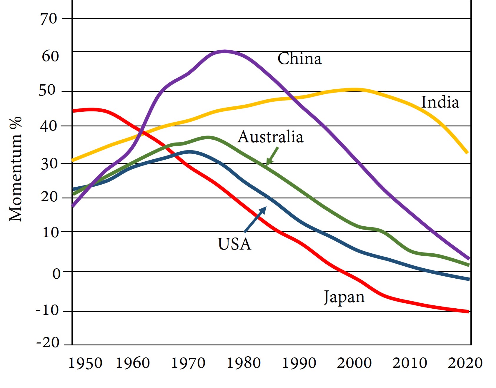
In Figure 14-1 below, the purple line represents the tendency of China’s population to grow just because there is a high proportion of the population that is of childbearing age.  This is known as population momentum.  Figure 14-1 indicates that during the years of China’s One Child Policy (1979-2021), population momentum was falling, but it was still positive.  According to the graph, China’s population was expected to continue to grow through 2020 because of  the positive momentum provided by China’s age structure.  Indeed, China’s population did grow until 2021.

We might consider what would happen to a population that is shrinking if its fertility rates suddenly jumped to the level consistent with an intrinsic rate of natural increase equal to zero. That population would continue to shrink for a while before stationarity was achieved, because the number of people of child-bearing age is lower than what it eventually will be.

Population momentum is the degree to which a population – if fertility rates suddenly changed so that its intrinsic rate of natural increase became zero – would continue to grow or shrink before reaching its stationary size.  We could alternatively say that population momentum is expected population growth ( or decline) that comes only from the maturation of different age groups before the stable age structure is achieved.

There are different ways to measure population momentum. One way is:

If this ratio is a number greater than 1, population momentum is positive, and even if the population’s rate of natural increase were to become zero, the population would still grow for a while before settling down to zero population growth (ZPG). If the ratio is less than one, population momentum is “negative”, with shrinkage expected before ZPG could be achieved.

Figure 14-1 uses this method, but records a population momentum value of 1.6 as “60”, meaning that the stationary population will be sixty percent higher than the current population at the given date.

Another way to quantify momentum is to see whether this fraction is greater than or less than one:

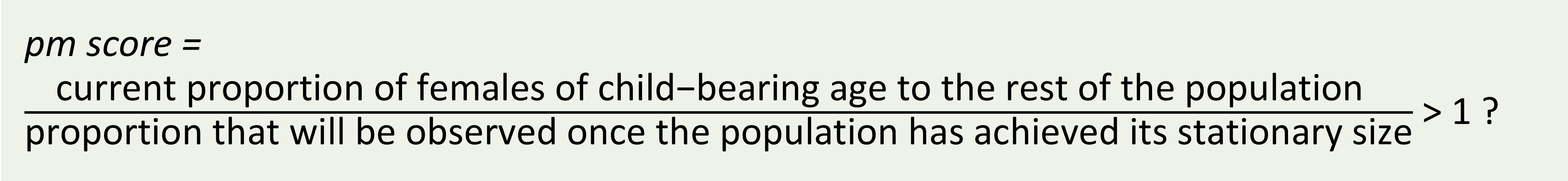
If this score is greater than one, then we have population momentum; if less than one, we have negative population momentum.  If the score equals one, we have no population momentum.  This approach to measuring population momentum will not be applicable to extreme situations such as the population being composed entirely of newborns.

The United Nations has used this rough ratio in the past:

Figure 14-2 below shows us that, in 2017, the United Nations projected the world population to reach over 11 billion by 2090 because of three factors:  decreases in mortality, fertility rates remaining higher than those compatible with stationarity, and population momentum.  Figure 14-2 indicates that even if mortality rates immediately froze and even if fertility immediately dropped to the level that would eventually stabilize the population at zero population growth, the world population would still rise to 9 billion people just because of population momentum.

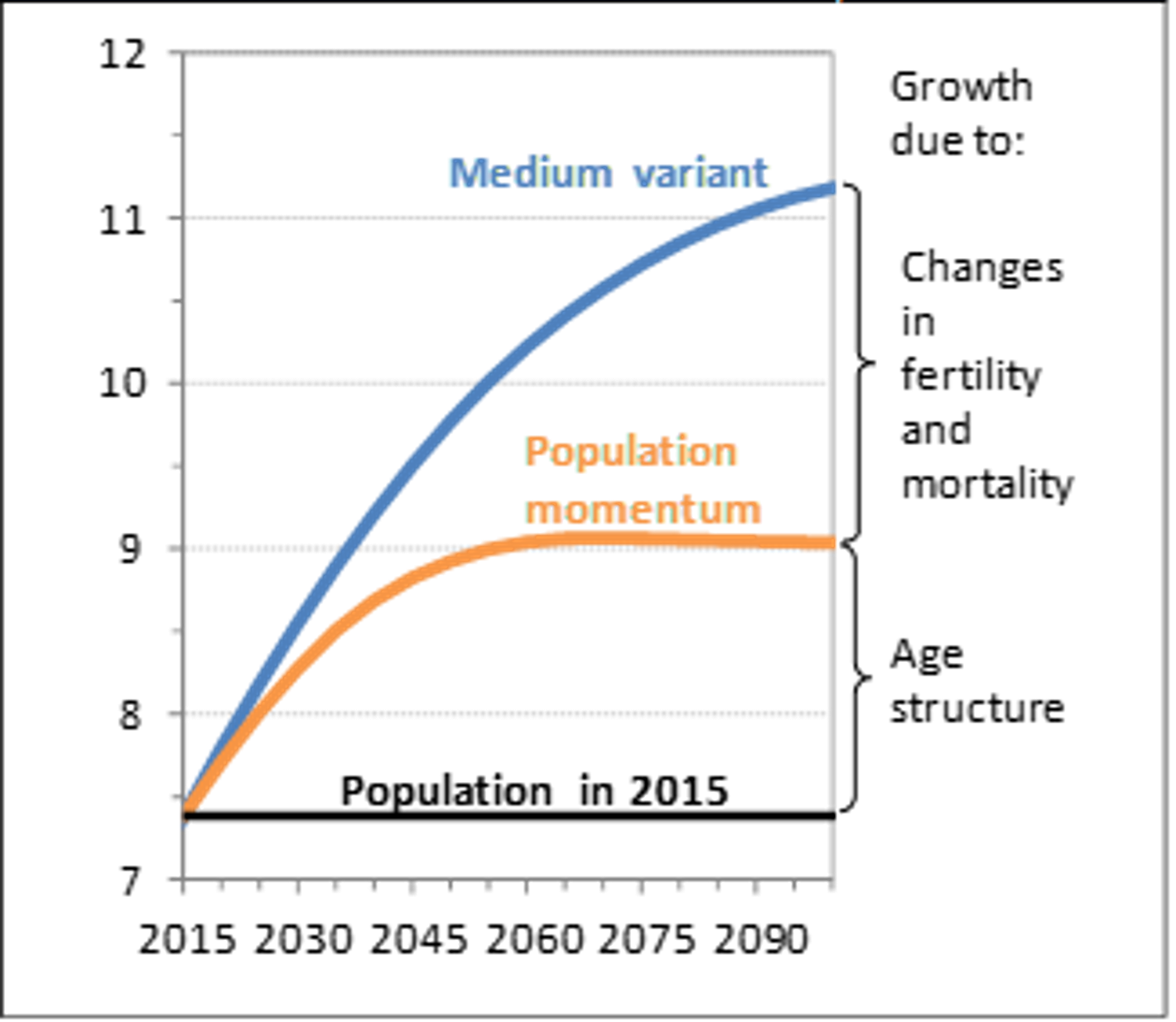
Figure 14-2 shows the “medium variant”, the predicted level of population growth using medium levels of fertility and mortality rather than the highest or lowest possible values.  The “momentum variant” is that portion of medium population growth that is due to population momentum alone.

We can predict a stable population’s eventual age structure.  One way is to use vectors and matrices to organize and manipulate the fertility and mortality information.

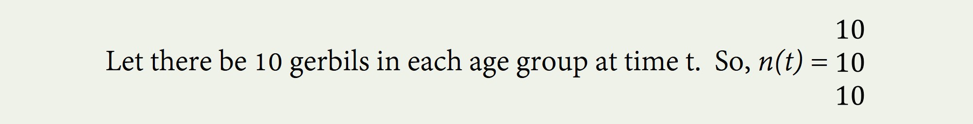
Let n(t) be a vector with s number of rows and one column. Each row represents an age group at time t. There are s number of age groups. The numbers in the each row represent  the number of gerbils, say, in each age group. Perhaps there are only three age groups:  newborns, age 1, and age 2.

For simplicity, we will not distinguish between male and female gerbils.

To figure out how fast this population will grow, and what the stable age mix will be, we need to know how quickly the gerbils reproduce, and what their survival rates are.  (Note that the survival rate is simply the number one minus the mortality rate. For example, 60% mortality during the year means 40% chance of surviving.)

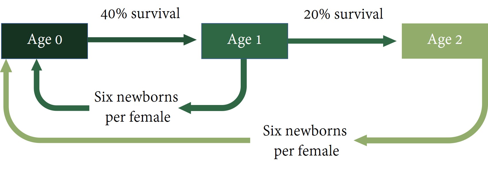
Let’s use a simplified description of gerbil life.  Perhaps newborns have a 40% chance of surviving until age 1. Perhaps one year-olds have a 20% chance of surviving until age 2. Perhaps two year-olds have a 0% chance of surviving until age 3. Perhaps newborns cannot reproduce, but female one year-olds have on average 6 live newborns during the year, and female two year-olds have on average 6 newborns also. Figure 14-3 below illustrates this.

In this example, all the age groups are related.  Not only do surviving one year-olds become two year-olds, but one year-olds generate newborns. Such a set of relationships lends itself well to matrix algebra and will result in a stable age structure.

The fertility and survival information summarized in Figure 14-3 above can be packed into a matrix with s number of rows and s number of columns.  Such a matrix, denoted by the letter “A”, is called a Leslie matrix.  We use the Leslie matrix to transform n(t), the age vector for year t, into n(t + 1), the age vector for year t + 1.

The first row of the Leslie matrix contains the fertility information: 0  3 and 3.  The zero in the first column means that newborns cannot have babies.  The 3 in the second column means that one year-olds have 3 babies each.  Note that we say 3 babies each, not 6 babies each, because although there are 6 newborns per female, only half the gerbils are female; on average there will be 3 newborns per adult gerbil.  For simplicity, we are not distinguishing between males and females.

The first row tells us that newborns have 0 babies each, one year-old gerbils have 3 babies each, and two year-old gerbils have 3 babies each as well.

Basically, each column belongs to an age group, with the leftmost column representing the youngest age group. The first row is the fertility row, showing how many babies are contributed per gerbil in each age group. The subsequent rows are survival rows. The second row/first survival row shows what percentage of gerbils make it from newborn (the first age group) to one year old (the second age group).  It reads 0.4, 0, 0  which communicates that 40% of newborns make it to age 1, zero one year-old gerbils turn 1, and zero two year-olds turn 1. The last row shows how many gerbils make it to the last age group, age 2.  As you can see, zero newborns turn 2, 20% of one year-olds turn 2, and zero two year-olds turn 2.  There is no subsequent row because all gerbils in the last age group die.

We’ve assumed that these gerbils never live past age two. In real life, gerbils can live longer than that.

To find how many babies there will be next year, which is the first number we need for our n(t+1) age matrix, we multiply the fertility row in the Leslie Matrix by the age vector n(t).  That means we multiply the first item in the fertility row by the first item in n(t), add that to the the second item in the fertility row multiplied by the second item in n(t), and add that to the third item in the fertility row multiplied by the third item in n(t).

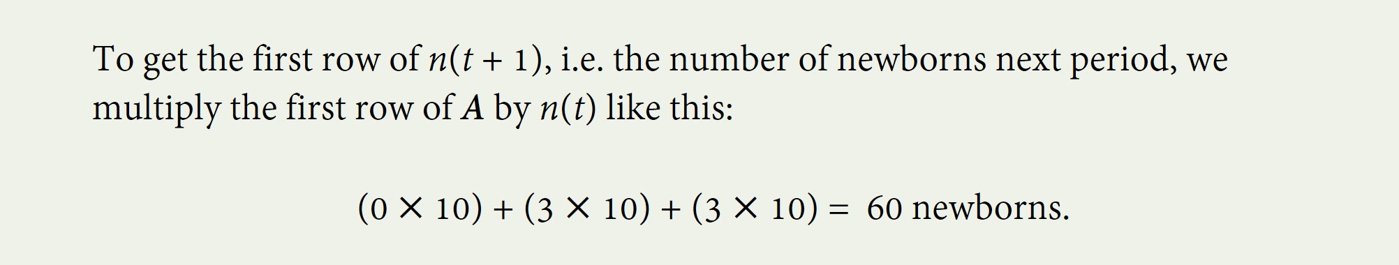
Our calculation shows us that newborns do not give birth to any newborns, but the 10 one-year-olds (male or female) give birth to an average of  3 babies each, as do the 10 two year-olds.

To find out how many one-year-olds there will be next year, we multiply the second row of A by the age groups in n(t).

Multiplying the rows in A by the columns in n(t) is the correct way to perform matrix algebra.  Always keep the Leslie Matrix A to the left of n(t), because, according to the laws of matrix algebra, the number of columns in the first object has to equal the number of rows in the second object.

Let’s continue with our example, using our first Leslie Matrix with ages newborn, 1, and 2.  We saw that, when we begin with 10 gerbils of each age, 60 gerbils are born and enter the newborn category.

How many one year olds will there be in n(t+1)?  Since only 40% of the original ten newborns will survive to age 1, and since the original 10 one-year-olds and the original 10 two-year-olds cannot turn one, there will be four one-year olds at n(t+1).

Finally, to find out how many two-year-olds there will be in n(t+1), we must multiply the third row of A by n(t) to find that there will be 2 two-year-olds next year.  0 x  10 + 0.2 (10) + 0 (10) = 2.

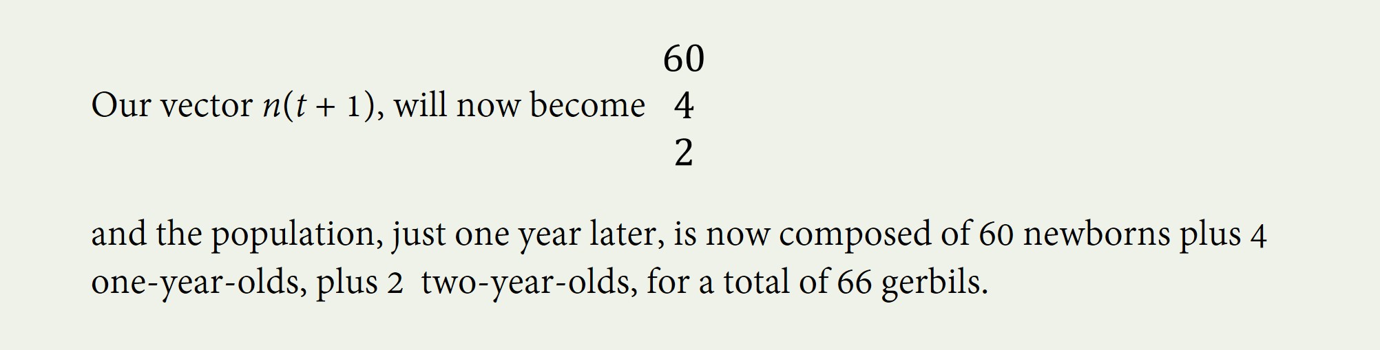
That’s a big difference in our gerbil population’s age distribution in just one year!   Not only has the population more than doubled, but the population has become much younger!  Magically, the age structure will eventually stabilize, usually in fewer than 70 periods.  When the age distribution stabilizes, the population’s growth rate – and the growth rate of every single age group – stabilizes too.

The point of writing the population’s dynamics in matrix form is that, once it is in matrix form, it is very  straightforward to compute what will happen to the population in the distant future.

To find what the population will look like in 70 years if present fertility rates and survival rates continue,  compute:

A computer can do this easily.

One can also find, using a computer or using matrix algebra, the eigenvalues of the Leslie Matrix A.  An eigenvalue is a number λ  that, together with some non-zero vector v(t), can “take the place of” matrix A in the equation:

The largest, positive, real eigenvalue happens to be related to the intrinsic rate of natural increase! Take the natural logarithm of this eigenvalue and you have the intrinsic rate of natural increase/decrease.

Another way to calculate the intrinsic rate of natural increase is algebraic, using the survival and reproduction rates.  This calculation is very complicated.^[1]

The gerbils in our example settle down to their stable rate of population growth after 56 years.  At that point and ever after, they experience r=0.1843 or eighteen-and-a-half percent population growth per year.

Once we have the intrinsic rate of growth, r, we can predict the stable age structure. We do this in Table 14-1 for our hypothetical gerbil population.  Again, we will ignore differences between males and females for simplicity.  The number of individuals in any age group x is related to the number of newborns x years ago multiplied by the exponential population growth factor (e^xr)and the relevant survival rates.

Call the number of newborns NN. Since the gerbil population (and every age group) is now growing steadily at e^0.185, there must have been  e^-0.185 fewer newborns last year than there are this year. 40% of those newborns would have survived the intervening year, giving us NN x e^-0.185 x 0.4  = 0.3324 NN one year-olds now.  That is to say, for every newborn, there are 0.3324 one year-olds.  This is recorded in column 3 of the Table below.

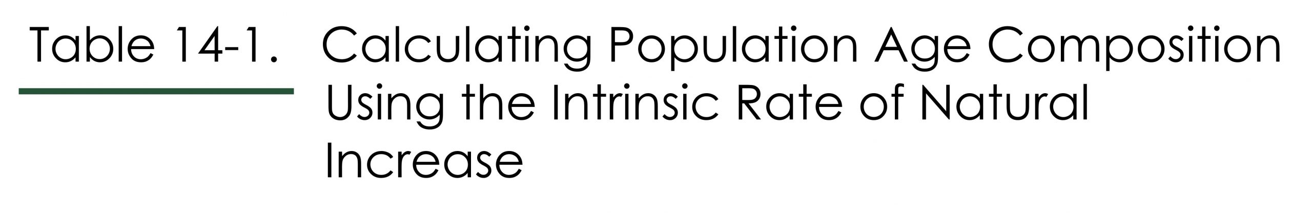
Column 3 of Table 14-1 gives us the number of gerbils in age category, expressed in terms of the number of newborns.  Adding up the gerbils in each column 3, we see that the total population, once stability has been achieved, will be equal to 1.3877 times the number of its newborns.  That is to say, the fraction of the population that is newborn is always 1/1.3877 or 0.72.  The stable age distribution is 72% newborn, 24% one year old, and 4% two years old.  We started with 33% of the population being newborns, 33% one year-olds, and 33% two year-olds, but once they were free to live their lives, reproduce, and die, the population converged to the 72:24:4 stable age distribution and to an intrinsic rate of natural increase of 18.5% every year.

Figure 14-6 below shows us that, after only 25 years or so, the gerbil population’s age structure settles down to the 72:24:4 age distribution. The dark blue (top) line represents the share of newborns, the reddish line represents the share of one year-olds, and the bottom grey line represents the share of two year-olds.  Initially, each group represented 33% of the population, since there were 10 of each age.

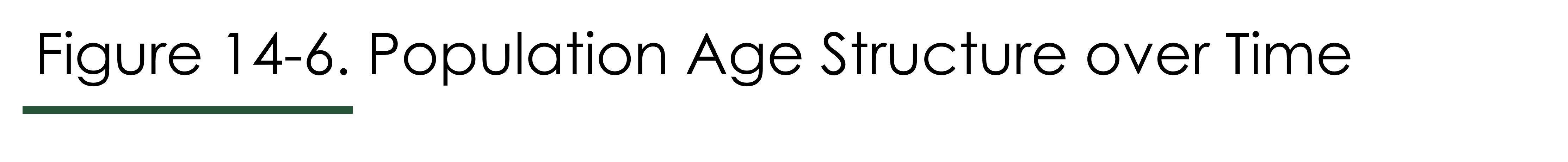
Why does this population of gerbils gyrate up and down during the early years?  It has to do with the inability of newborns to reproduce.  At time zero, when one year-olds and two-year olds make up a majority of the population, many newborns will be generated for next year, so year 1 will see newborns become by far the majority (recall Figure 14-5).  But these newborns cannot yet reproduce, so the fraction of the population which can reproduce in year one is smaller that it was at year zero.  Consequently, newborns in year two will not be as dominant as they are in year one.  In year two we will see more one year-olds than newborns. Meanwhile, one and two year-olds are experiencing heavy mortality, making it less and less likely over time that they can form a majority of the population.

So far we have used the Leslie matrix to predict what a population will look like once it stabilizes.  But the Leslie matrix has a more general application.  We can use the Leslie matrix to predict what a population will become in the future, even if fertility and survival rates are changing.  We’ll just have to keep updating our Leslie Matrix with the fertility and survival rates that apply to the year in question.

Application of the Leslie Matrix to the history of Ukraine

Let’s move from discussing gerbils to discussing human history.  Vallin et al. (2002) wanted to count crisis deaths in the Ukraine during the 1930s and 1940s. The problem was, no death statistics for Ukraine had been published between 1931 and 1954.  Vallin and team found a solution.  They began with a 1926 census of Ukraine.  To predict how many people should have been alive in 1939, when there was another census, they applied a Leslie matrix or similar computations to the initial 1926 population age vector.  For their Leslie matrix or similar computations they used survival rates from a model Life Table, representing countries which were similar to Ukraine but not experiencing crises.  The difference between the projected number of people in 1939 according to their calculations, and the actual number in 1939 according to the census, gave them the number of missing people.  They did the same thing between the 1939 and 1959 censuses.

There are three reasons that the actual population in a later census would be smaller than the population in an earlier census projected forward, three reasons why people would be missing.

The first reason is that some people left the country.  A Leslie matrix does not deal with this possibility. The second reason is that fertility was actually lower than what was assumed when making the projection. And the third reason is that mortality was actually higher than was assumed when making the projection. Crises can cause extra deaths, extra emigration, lower immigration, and lower fertility.

Vallin et al. had used model Life Table survival rates to project the population.  They had also made a conservative (i.e. low) estimate of what fertility would have been without the crises.  If anything, this low-ball estimate of what fertility would have been without the crisis would underestimate the reduction in births due to the crisis. Vallin et al.’s approach can be summarized as follows.
STEP ONE

Project the population in 1926 forward to 1939 using 1926 census data for the initial population age vector, and using a  Leslie matrix or similar procedure.  The Leslie matrix is supplied with non-crisis age-specific survival rates from a model Life Table, and non-crisis fertility rates from similar countries.

subtract the actual population in year 1939

= total population loss (due to crisis deaths, births foregone due to the crisis, and net emigration)

STEP TWO

project the population in 1926 forward using 1926 census data in the initial population age vector and using a Leslie matrix with non-crisis age-specific survival rates but using estimated actual fertility rates

subtract actual population in year 1939

= population loss due to crisis deaths and net emigration

The difference between this and total population loss calculated earlier is the number of births foregone.

STEP THREE

Take your estimate of population loss due to crisis deaths and net emigration and

subtract estimates of net emigration 

=population loss due to crisis deaths

By following these steps, Vallin’s team was able to divide population loss between its three different causes.  They concluded that  although Ukraine’s population grew between 1926 and 1939, it was smaller than it should have been, by 4.6 million people.  That’s on a base population of 29 million in 1926. Approximately 0.9 million people left the country, 1 million people were not born because of the crisis, and 2.6 million people died because of the crisis.

In this chapter we learned about stable and stationary populations, and how a constant age structure emerges when fertility and mortality rates are constant.  We learned how to project populations forward using a Leslie matrix.  We will now spend a few chapters discussing real-life changes in fertility, mortality, and the age structure.

1. You are given the following information for a population of gerbils.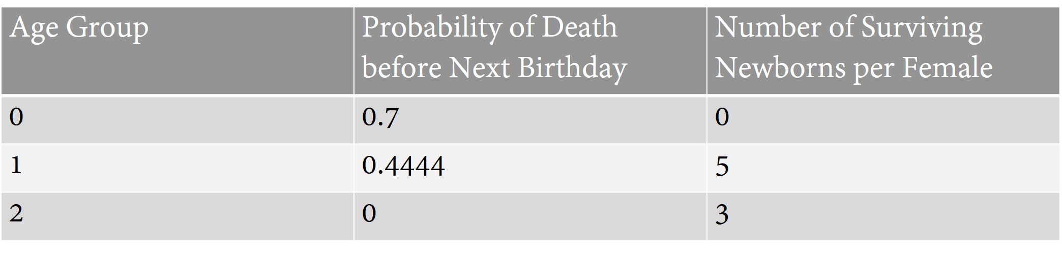

a) Write the population projection matrix A that could be used to describe the mechanics of this population of gerbils.

b) If, initially, there are 100 gerbils age 0, and no other gerbils, what will the age vector, n +1, be in the next period?

2. Given this population projection matrix,

3. Consider a different population of gerbils with the same survival probabilities as have been given in question 2. You are told that the intrinsic rate of population decline for this new population is 5% per year. What is the stable age mix of this population (before it disappears!) What would the stable age mix be if the intrinsic rate of population growth was 5% per year?

4. If a population of gerbils is growing at 2%, and the population is stable, how fast is the population of newborn gerbils growing?

5. In a population of hamsters, 63% of the population is newborn, 24% are one year-olds, and 13% are two year-olds. Fertility is equal to 8 surviving young per female less than 1 year old, 16 surviving young per female over age 1 but less than two years old, and 4 surviving young for two year-old gerbils. This, however, is not the stationary situation. Imagine you calculate that, in the stationary situation, 61% will be newborn, 24% one year-old, and 15% two-year olds.

a) Is population momentum greater than one or less than one?

b) Will the population grow or shrink before it achieves its stationary size?

c) What kind of immigration or emigration could hasten achievement of the stationary population size?

6. If the population of polar bears in southern Hudson Bay is 1,000, and the projected stationary population is 800, what is this population’s momentum? What must be true about the current age structure in the population?

7. Looking at Figure 14-1 in the text, we see that momentum was increasing in China prior to 1980. What does this mean?