
In Chapter 3 we learned how to calculate the crude death rate. We divide the number of deaths by the midyear population, then multiply by 1000 for convenience. Because the crude death rate has population in its denominator, it automatically adjusts for the fact that larger populations will have more people dying. There is no reason that a large country must have a higher death rate than a smaller country.
Population size does not directly affect the death rate, but having a lot of older people in your population does.
Japan has an older population than Afghanistan, so old that Japan’s 2019 crude death rate, 11 per 1000, was higher than Afghanistan’s crude death rate, 6 per 1000. This makes Japan look like a less healthy and more dangerous place to live than Afghanistan. Is it?
No. At every age of life, the 2019 age-specific mortality rates were lower in Japan than they were in Afghanistan. A twenty-year old in Afghanistan had a higher chance of dying that year than a twenty-year old in Japan. However, a twenty-year old in Afghanistan did not have a higher chance of dying that year than a fifty-year old in Japan. And Japan had a higher fraction of its population age 50 or older than Afghanistan did. That’s why Japan’s crude death rate was higher than Afghanistan’s, and why the crude death rate can be misleading when comparing countries.
Let’s learn how to transform a crude death rate into a standardized death rate. We’ll use the Table below.

Table 5-1 shows us the actual number of deaths from COVID-19 in Taiwan and Japan as of September 30, 2020. By that date, Taiwan had experienced a total of 7 deaths, 2 from 25-49 year-olds, 4 from the 50-74 age category, and 1 person age 75+. If you divide those 7 deaths by Taiwan’s population of 23,562,323 people, then multiply by 1000, you get a crude death rate for Taiwan of 0.0003 deaths per 1000 people, or 3 deaths for every ten million people. Clearly, Taiwan was doing very well.
Japan wasn’t doing too badly either, with a crude death rate of 125 per ten million people, but its crude death rate was about 40 times as high as Taiwan’s.
Now let’s standardize the death rates. To do so, we are going pretend that each country has the same, standard age distribution. What is this standard age distribution? Often, the United States population is used as the standard. Or we could use the World Health Organization’s “World Standard Population”, which is an estimate of the age distribution of the entire world.
In this example, we are going to choose Taiwan’s age distribution as the standard. Taiwan will be our “reference country”.
Since Taiwan already has Taiwan’s age distribution, we don’t have to do anything to its data. Taiwan’s death rate, standardized to itself, will simply be its original crude death rate of 3 per million.
However, Japan’s standardized death rate will be different from its crude death rate.
Step 1 of finding Japan’s standardized death rate is to find the number of people of each age who would have died in Japan if Japan had had Taiwan’s population. For each age group, we take the Japanese mortality rates (second-last column) and multiply by the number of people that age in Taiwan (3rd column). This gives us the last column in the table. We see that, if Japan had had the population of Taiwan, nine 25-49 year-olds would have died, seventy-nine 50-74 year-olds would have died, and eighty-five people age 75+ would have died.
Step 2 of finding Japan’s standardized death rate is to add up all the deaths in that last column and use it to find the overall death rate. The nine 25-49 year-olds plus the seventy-nine 50-74 year-olds plus the eighty-five people age 75+ who died add up to 173 deaths. We then divide those deaths by the total population (using Taiwan’s population) and multiply by 1000. This gives us the standardized death rate of Japan, standardized relative to Taiwan’s population.
Japan’s new, standardized death rate is 73 per million, less than its crude death rate of 125 per million. If Japan had had Taiwan’s younger population, fewer people would have died. Japan’s crude death rate was misleadingly high. It made Japan look like it was dealing with COVID-19 less well than it actually was. The large fraction of elderly in Japan was biasing the crude death rate.
To repeat, standardizing to Taiwan’s population, Japan’s death rate falls from 125 per million to 73 per million. Its death rate is still higher than Taiwan’s but the difference is not as great as before, showing that part of the reason Japan’s crude death rate was higher than Taiwan’s is that Japan had a higher proportion of older adults.

A student once reported that Japan’s COVID-19 death rate, if standardized to Taiwan’s population, would fall, while Taiwan’s COVID-19 death rate, if standardized to Japan’s population, would also fall. In other words, standardization made both countries look better relative to each other.

The reason the student got this result is that they had collected the wrong data. They reported that, in Japan, most people who died of COVID-19 were older adults (TRUE), but in Taiwan, most people who died of COVID-19 were young adults (FALSE). If both statements had actually been true, then giving Japan Taiwan’s younger population would indeed make Japan’s COVID-19 death rate fall, and giving Taiwan Japan’s older population would indeed make Taiwan’s COVID-19 death rate fall too.
Though most people who died of COVID-19 in both Japan and Taiwan were older adults, it’s possible that a disease could impact different age groups differently in different countries. Simply standardizing by the age distribution of one of the countries’ populations would not be meaningful in that case. We would have to form a reference population more creatively, as the following example shows.
Sudharsanan et al. (2020) age-standardized the COVID-19 Case Fatality Rate in different countries, studying deaths from COVID-19 in nine countries up until April 19, 2020. (The Case Fatality Rate, or CFR, is the percentage of people who die once infected.)
To begin, Italy had the worst crude Case Fatality Rate (CFR), at 9.2%. That means 9.2% of people who caught COVID-19 died. By contrast, Germany’s crude CFR was only 0.7%. Once the case fatality rates were standardized to a reference population, however, the gap between Italy and Germany shrank: Italy had a standardized CFR of 3.9% compared to 1.3% for Germany. Italy’s and Germany’s CFRs weren’t as far apart once the authors adjusted for the average age distribution of the people who were infected. In Italy, the people who got infected tended to be significantly older than the people who got infected in Germany.
The authors didn’t use any one country’s age distribution as the reference population. The authors used the nine countries’ average age distribution of people who actually got infected as the reference population.
They found that 66% of the difference in countries’ crude case fatality rates arose from the countries having different age distributions of people infected.
After standardizing this way, Italy was still in last place but not by as much. Switzerland, the Netherlands, and France improved their rankings while Germany, the US, South Korea, China and Spain slipped.

If you add the crude birth rate (per 1000) and subtract the crude death rate ( per 1000), and add on the net migration rate (per 1000), you will have the rate of population growth (per 1000); however, this rate of population growth is relative to the midyear population. That’s because the crude birth rate, the crude death rate, and the net migration rate are all evaluated per 1000 people at mid-year.
The way population growth is usually described is as a percent increase or decrease from the initial, beginning-of-year level.

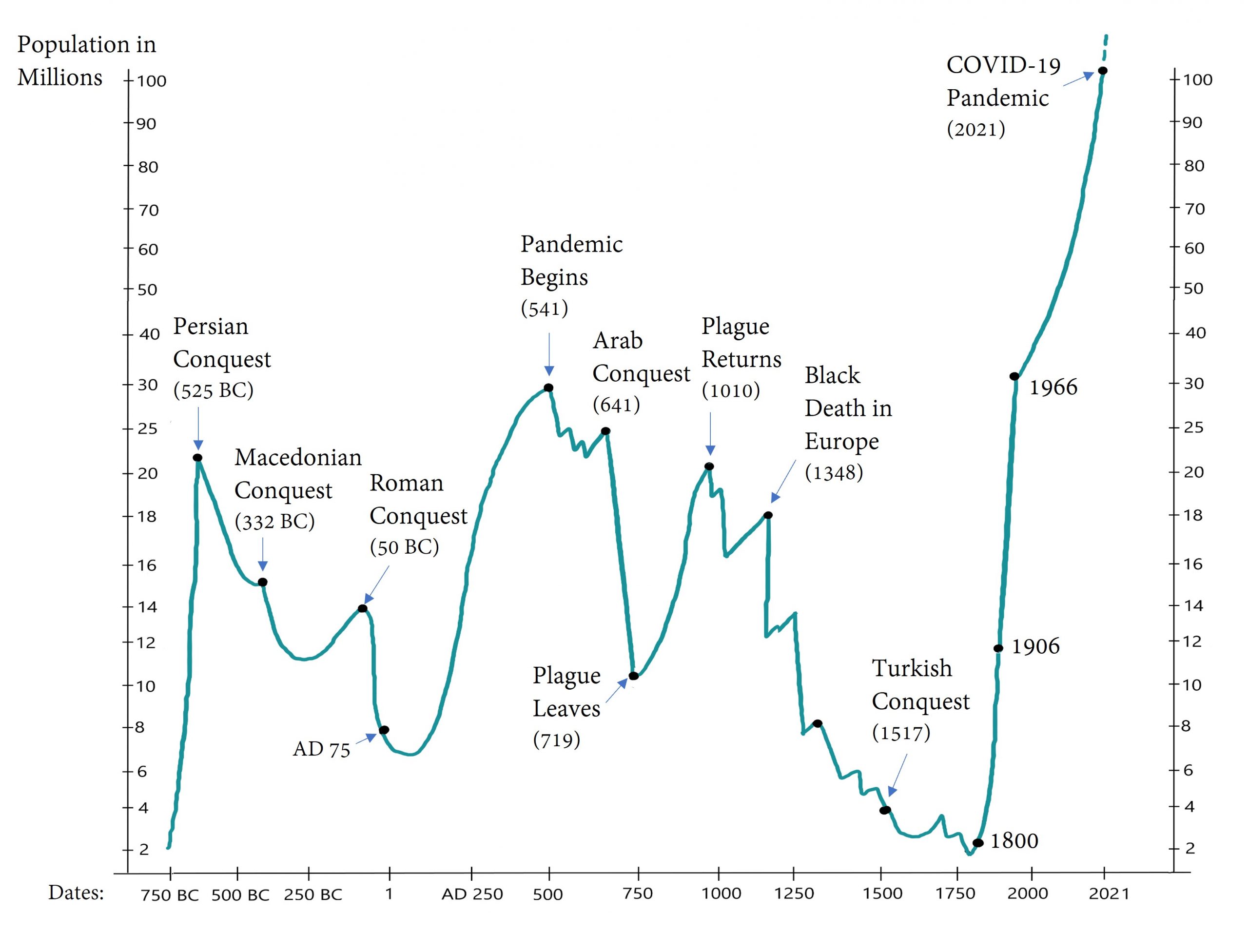
The population growth rate can fluctuate as a consequence of changes in fertility, mortality, and migration. Fertility, mortality, and migration can change for many reasons, such as war and famine. See Figure 5.1 to see how the population of Egypt, and the rate of growth of the population of Egypt, fluctuated over time.

“In the twentieth century, dire warnings and apocalyptic forecasts for the planet followed from the assumption that a particular pattern of increase…would persist in the future. The twentieth century also brought forth national population decline, or at least a fear of it, as a recurring theme in some more developed [sic] countries… Assumptions about constant rates leading to extinction, however, will be as untenable as those about constant rates creating ever burgeoning numbers.”
The three kinds of constant growth in math are arithmetic, geometric, and exponential growth. They are shown in the Figure below.

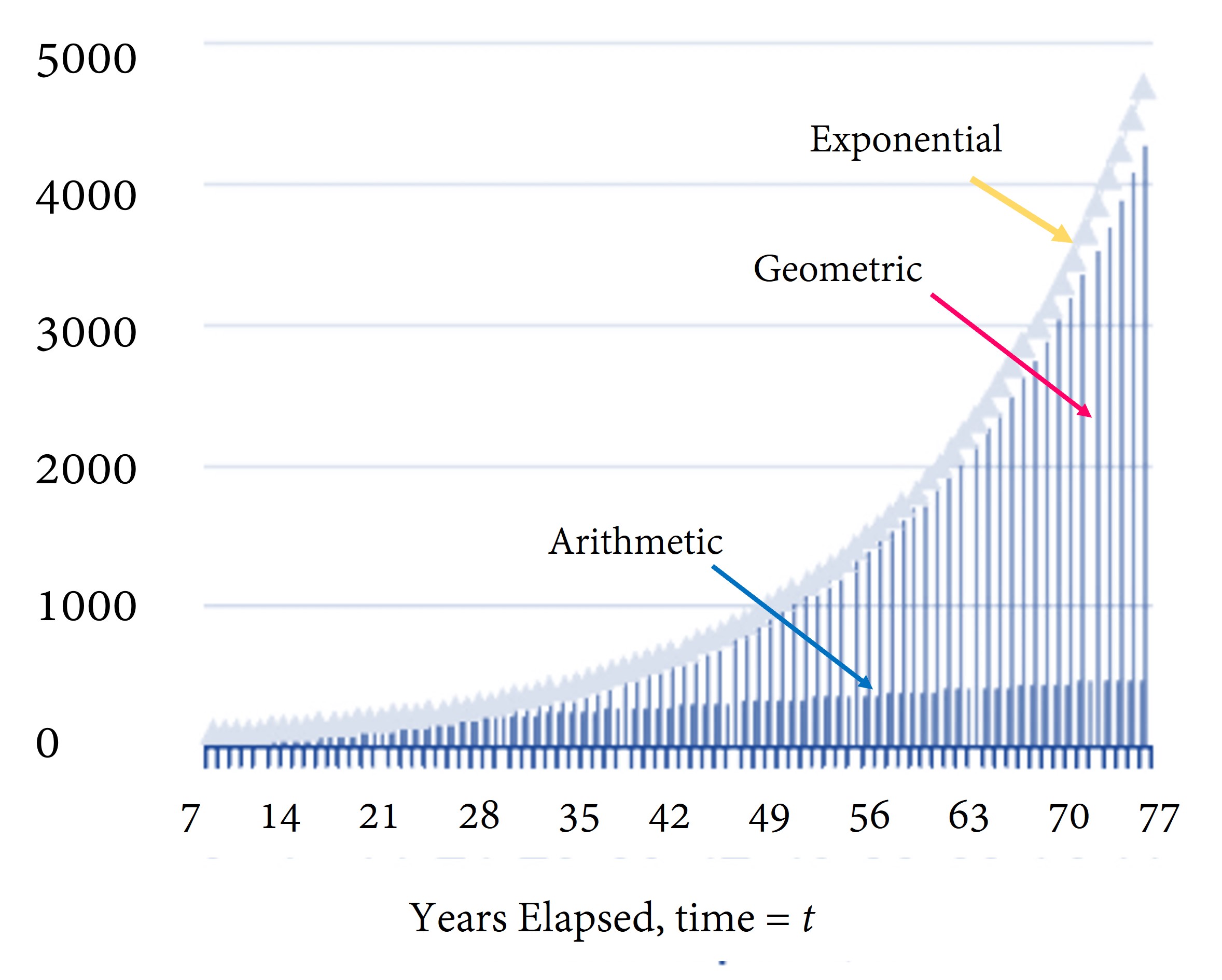
Arithmetic growth is steady. The increase in numbers is constant each year. Graphed over time, population grows with a constant slope.
Geographic and exponential growth are not steady over time. The larger the population becomes, the greater the increase in the population.

In the context of height, arithmetic growth means growing a set number of inches per year regardless of how tall you already are. It is like earning a fixed amount of interest each year: the interest does not compound, but is paid only against the initial amount deposited.
Malthus assumed erroneously that agricultural output could only grow arithmetically, for example by people clearing a fixed number of additional acres of land each year.
Malthus knew that population does not grow arithmetically, but in proportion to the base population. Nevertheless, we sometimes use the assumption of arithmetic population growth, especially for short time periods.
For example, to find the mid-year population, we simply assume that population was growing arithmetically during the year: we sum the population at the beginning of the year with the population at the end of the year, and divide by two.
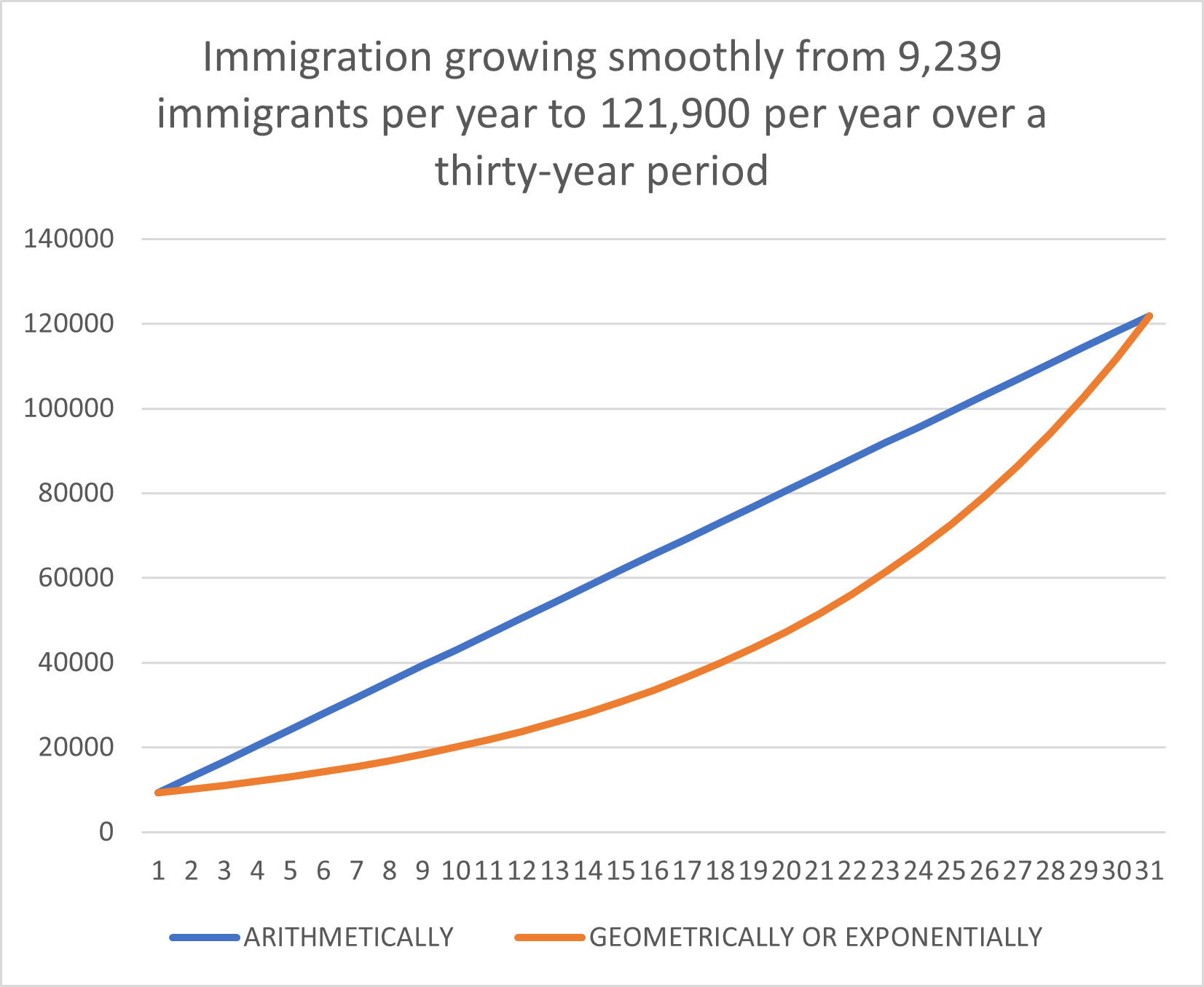
Demographers often use the assumption of steady growth when estimating what happened between two historical periods of time for which they have data. For example, if all we knew was that in 1941, 9,239 people immigrated to Canada and that in 1971, 121,900 people immigrated to Canada, we might assume, in the absence of other information, that immigration grew steadily during that time. We might assume it grew steadily in an arithmetic way, a geometric way, or an exponential way. Over such a short period of time, there would not be much difference between the geometric and the exponential growth path, as shown in the Figure below. The geometric path would be a series of step functions, flat during a year, then rising at the beginning of the following year, while the exponential path would be completely smooth.

The arithmetic growth path can be found by subtracting the 9,239 immigrants in 1941 from the 121,900 immigrants in 1971 and dividing the difference by 30 to get 3,755.4 extra immigrants every year. 9,239 immigrants in 1941, 9,239+3,755.4 new immigrants in 1942, that number plus 3,755.4 in 1943, etc.
In year 1941+t, the number of newly arriving immigrants would be y = 9,239 + 3,755.4*t
The arithmetic growth path is just a straight line with intercept 9,239 and slope 3,755.4.
To estimate the total number of immigrants that arrived during the period 1941-1971, we would find the area under that straight line, which is simply the rectangle 9,239 x 30 plus the triangle (121,900-9,239) x 30 x 0.5 for a total of 1,689,915.
What if we had assumed geometric growth or exponential growth? We see that the area under those curves is less than the area under the line representing arithmetic growth. (See Figure 5-3 above). Geometric or Exponential growth assumptions will give us a lower estimated number of total immigrants for the period. That’s because geometric growth and exponential growth take a while to get going.

Geometric growth is like growing a fixed percentage of your initial height each year. It is like the growth of your bank account when you are paid interest once a year, and the interest compounds over the years.
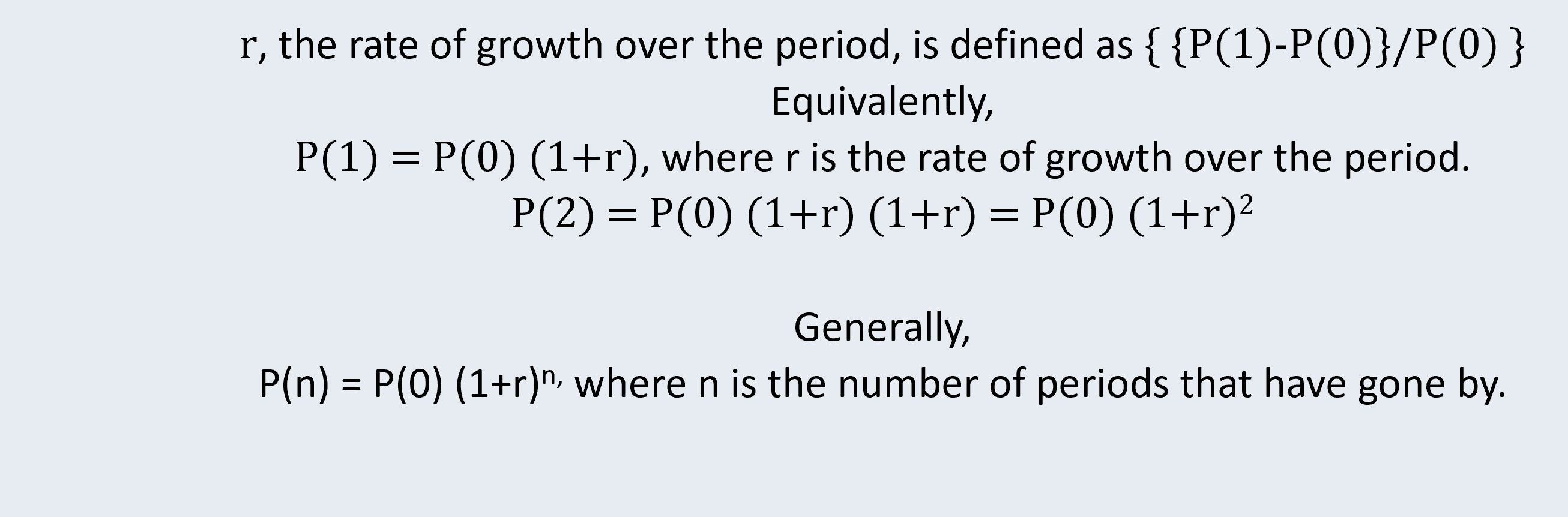
If we shorten the time between intervals when the growth is reckoned, we have continuous compounding i.e. exponential growth. “r” is still the official, annual rate of growth, but a fraction of it is implemented every second.
Exponential growth occurs when the interval at which growth or interest is compounded shrinks down to almost zero. It is like growing a tiny percentage of your height, every second, with your height being constantly updated. Exponential growth is smooth and continuous, which seems more realistic than geometric growth. However, real-life growth tends to come in spurts and fits, and there is certainly a turnaround time before a new baby can reproduce him or herself. So constant exponential population growth is not all that realistic an assumption.
Incidentally, Rowland (2003) points out that “The world’s population growth rate has never exceeded 2.1 per cent [per year] (doubling time 33 years), and the growth rate has been falling since the mid-1960s.”
A rate such as 2.1 per cent raises the question, 2.1 per cent of what? and lets you know that we are talking either about geometric or exponential growth. Usually demographers talk about exponential growth.


To find doubling time, simply divide the number 70 by the average growth rate per period. For example, if the growth rate is 2.1% per year, then the approximate time it will take for the population to double is 70/2.1 = 33.3 years. This is the “Rule of 70” which comes from the mathematics of exponential growth below:


Thus n, the number of periods required for doubling = ln(2)/ r ≈ 0.70/ r, where r is expressed as a decimal. (If using 70 instead of 0.70, r is not expressed as a decimal, but as a percent as in 70/2.1 percent = 33.3 years).
Getting back to our immigration example, if we assume that immigration grew geometrically from 9,239 people in 1941 to 121,900 people in 1971, we can solve for the annual rate of growth this way:


This is not very convenient to compute. It is easier to compute assuming exponential growth.
If we assume that immigration grew exponentially, we can solve for the rate of growth this way: How many people immigrated during the period? That would be:
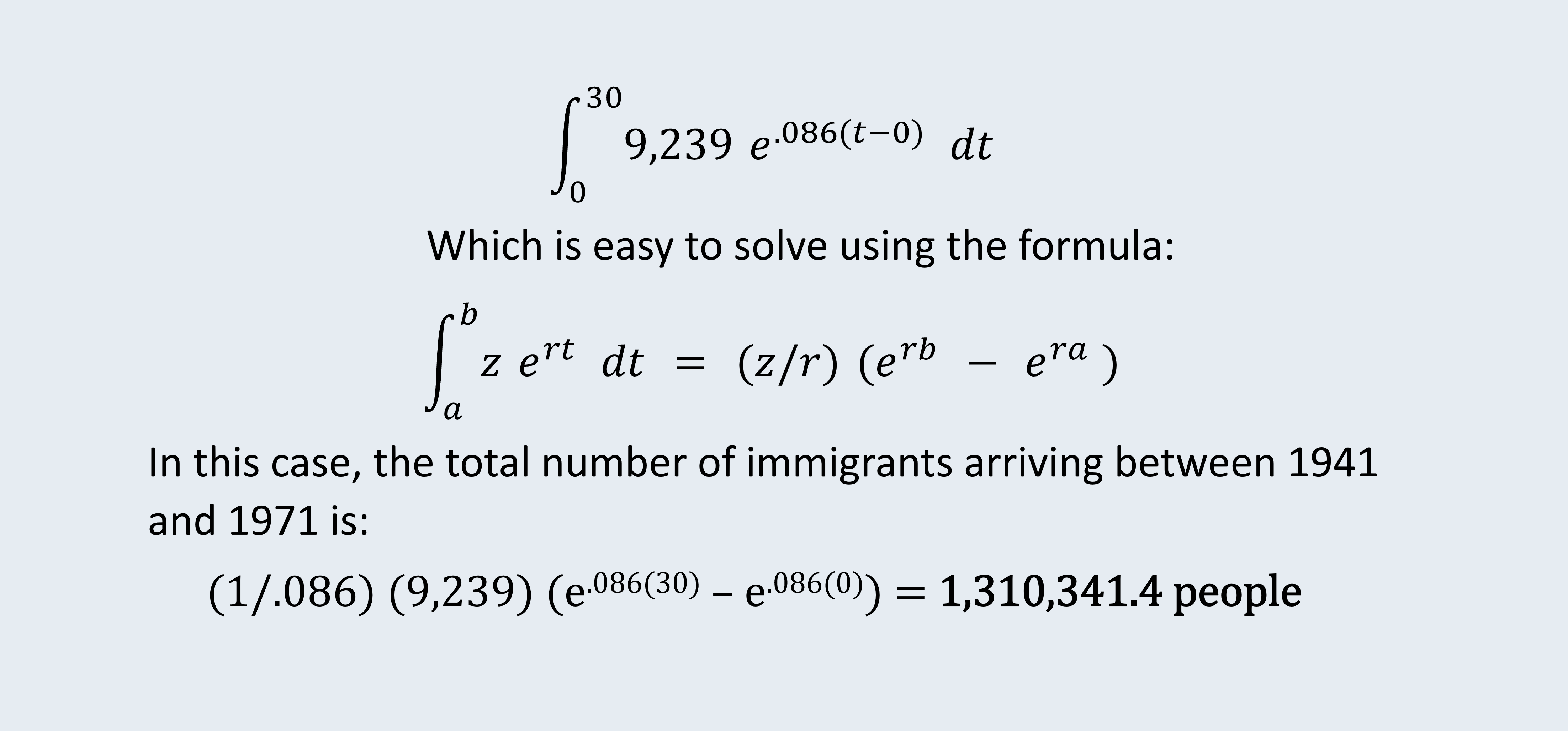
In real life, the number of immigrants who came to Canada between 1941 and 1971 was 3,597,689. In real life, the immigration rate was not smooth in any way, neither exponentially, geometrically, or arithmetically.
Does it seem funny that our exponential growth assumption resulted in the smallest estimate of total immigrants? Recall that really big gains from exponential growth are not evident for a while. Exponential growth takes a while to get going. That is true of geometric growth as well.
Exponential math has been used to estimate the number of people who have ever lived.

The Population Reference Bureau (https://www.prb.org) provides an up-to-date estimate of the number of people who have ever lived, and in mid-2020 it reckoned that the number of people alive represented 6.7% of the people who have ever lived.
If all of the people who have ever lived stood side by side, with a space of one square meter allocated per person, the entire human race would occupy an area approximately the size of modern-day Eritrea (117,600 sq. km)[1].

.svg)
In the next Chapter we will explore the concept of the life table and its importance for population economics.

1. Based on the following table, complete the questions:
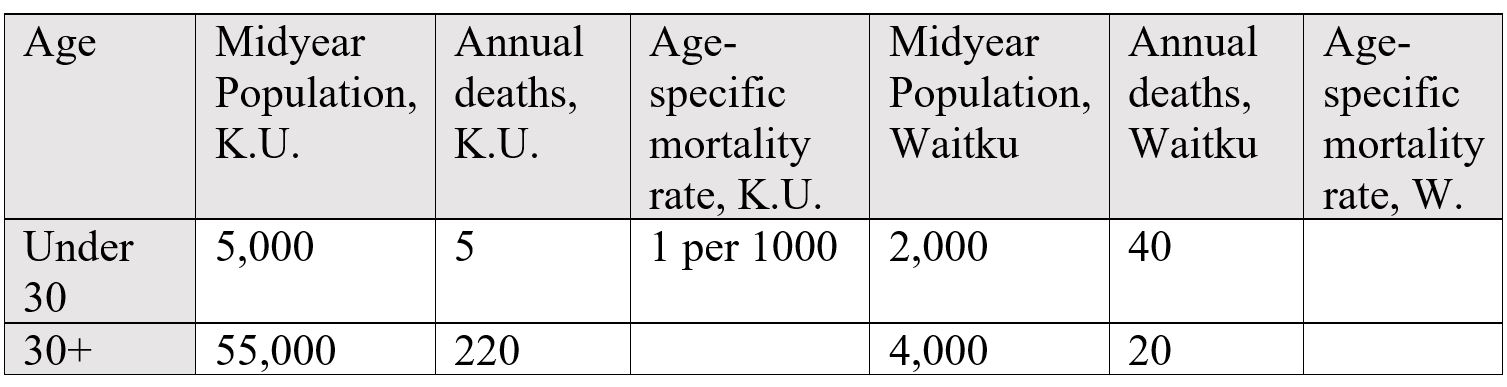
a) Fill in the blanks in the above table.
b) Using the information in the table, compute each country’s crude death rate, and also each country’s standardized death rate using K.U. as the standard/base country.
c) How does your impression of Waitku change once you perform the standardization?
2. If the sex ratio of 20-24 year-olds is currently equal to 1, and if the flu season results in many more 20-24 male deaths than female deaths, what will happen to the sex ratio in that age group?
3. Ignoring medical and other advances, what happens to a nation’s crude death rate as its population gets older? How could we adjust for this effect?
4. If the population of gerbils is 53,460 today, and the population has been growing exponentially at a rate of 2% per year, what was the population of gerbils 10 years ago?
5. How long will it take for this population to double?
6. At the time of creating this question, the world’s population was expected to grow from 7 to 8 billion in 13 years. What rate of exponential growth would that imply?
7. Consider a nation which had 100 people in 1900. By 1980 they had 500 people. At what geometric rate did this population grow? At what exponential rate did this population grow? At what arithmetic rate did this population grow?
8. If the number of births in 1900 was 1, and the birth rate grew at a 4% exponential rate, write an expression for the number of people born during 1900-1980. Solve for the number of people born during 1900-1980.
- https://mapfight.xyz/map/hn/#er ↵
Death rates can be adjusted to account for differences in countries that might bias the crude death rate. A death rate is that is adjusted in this way is called a standardized death rate. Death rates can be standardized for age, sex, or other factors.
Doubling time is the length of time it takes for a population (or anything else) to double. It can be approximated by the formula 70/r, where r is the growth rate expressed as a percentage.
