
So far we have not studied migration. Everything we have learned can apply to an isolated population. But very few societies are isolated any longer. Immigration and emigration pressures can greatly influence a nation’s standard of living and economic potential.
Usually when we speak of immigration, we mean legal migration across national borders. But the motives and consequences of migration are similar whether the movement is legal, illegal, across national borders, or just across the neighbourhood.
Governments tightly regulate immigration, but there are always some people who manage to enter illegally. Governments typically do not keep track of emigration. In this way both immigration and emigration pose measurement challenges.

If migration data are lacking, you can estimate the NMR using the demographic equation from Chapter 3. If you know the change in population, and births and deaths during the year, you can infer the rate of increase due to net migration. If further you know the immigration rate, you can infer the emigration rate.

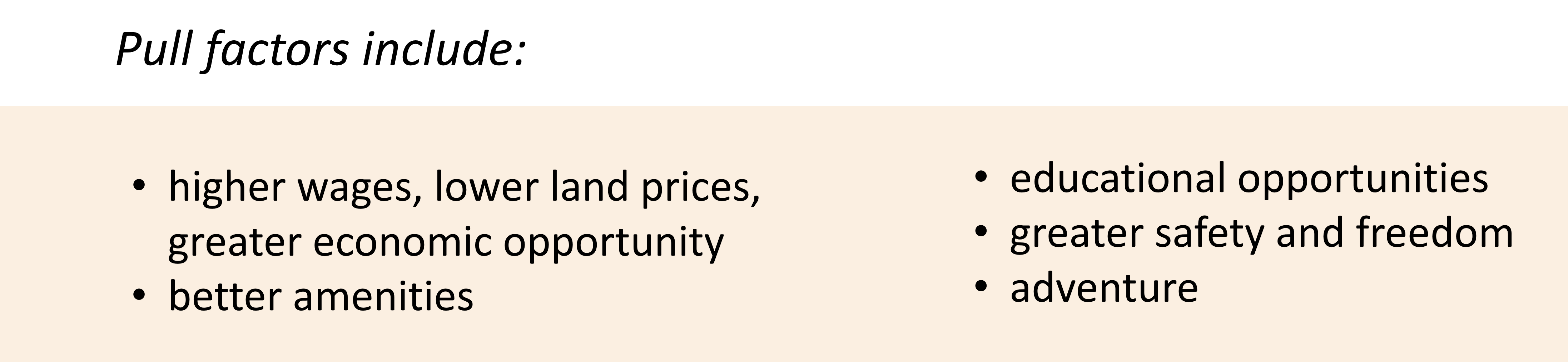
 People migrate because they are PUSHed out of their old place of residence and/or PULLed into their new place of residence. We’ll discuss the special push and pull factors associated with human trafficking and slavery in our next chapter. For people who are choosing to migrate,

Depending on the push or pull factors, those who migrate may share certain characteristics.
E.S. Lee (1966) emphasized that “migrants are not a random selection of the population at origin.” For one thing, migration is more likely at certain stages of life, such as graduation from an educational program, entering the labor force, leaving the parental home, widowhood or divorce, and retirement.
Abramitsky, Boustan, and Erikkson (2012) studied men who migrated from Norway to the United States in the late nineteenth century, men who had non-emigrating brothers. They found that households with poorer economic prospects were more likely to send migrants to the US, and that within households, men with poorer prospects were more likely to migrate. Men who migrated from rural areas ended up doing 93% better financially than their brothers who remained at home, whereas men from urban areas did 42% better financially after migrating.
Simone Wegge (2009) has studied data from more than 1000 villages in the German principality of Hesse-Cassel during 1852-1857. Her data suggest that, up to a certain point of wealth, people with more money were more likely to immigrate than those without. After all, the trip to New York from Hamburg cost twice the yearly wage of a labourer. But at the highest levels of wealth, there was not the incentive to emigrate. This suggests that regions with more polarization of income will experience less emigration.[1]. Wegge found that the villages which experienced the most emigration were those
- that practiced unigeniture: the eldest son would inherit the entire farm, leaving little for other sons.
- those which had higher emigration flows in the past
- those with fewer factories
- those with more religious minorities
When migration is voluntary, the people most likely to migrate are possibly:
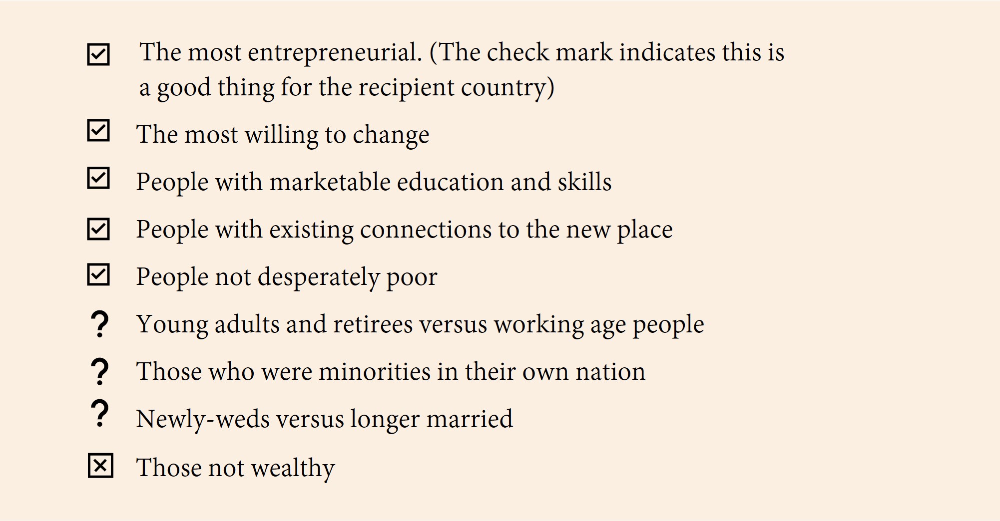
It is important to anticipate how an immigration policy and a global situation will select for a particular kind of immigrant.

The most important PULL factor tends to be the expected real wage in the destination country. It is not enough to know that the average wage is higher in the destination country than in the home country. A would-be migrant must divide the average after-tax wage in the destination country by the cost-of-living to find the after-tax real wage in the destination country, and that after-tax real wage must be multiplied by the probability (less than one) that he or she will succeed in finding a job.
The savvy migrant calculates the expected real wage, formed by multiplying each possible real wage (after income tax) by the probability of achieving it, and summing the total. The migrant then compares that expected real wage to what they are earning in the home country.
The same math works for migrants considering moving within a country between one region and another. This model, known as the Harris-Todaro model, was developed to explain rural-to-urban migration. It does not consider a region’s amenities, safety, or other factors, just the real wage that people can be expected to earn.
Consider a hypothetical city in which there are two sectors, a formal sector where wages are recorded and taxes are paid, and an informal sector where taxes are not paid. Let e1 be the probability that the migrant can find work in the formal sector. Similarly, let e2 be the probability the migrant can find work in only the informal sector, which is not recorded or taxed, presumed to be their second choice. The unemployment rate is 1-e1–e2.
As expressed in Equation 20-1, workers going to the city can expect to earn the formal sector after-tax real wage multiplied by e1, plus the informal sector real wage multiplied by e2, plus nothing at all or some welfare payment multiplied by the probability of not finding a job in either sector (1-e1–e2).
Equation 20-1. expected real wage in city = e1 x formal sector after-tax real wage + e2 x informal sector real wage +(1-e1–e2) x income available if unemployed
As workers stream into the city looking for work, the unemployment rate in each sector is likely to rise, and wages are likely to fall, at least in the short run, because more people are competing to work there. Thus the expected urban wage will fall until it is equal to the rural wage. At that point, moving to the city to earn a better wage is likely to be disappointing.
Equation 20-2. expected real wage in destination location = actual real wage in current location
Equation 20-2 tells us that in equilibrium, one city cannot offer higher expected real wages than another city. Migration to the city with the higher expected real wage would continue until its wages came down or its unemployment rate went up.
If the formal sector city wage cannot fall as low as the rural wage, perhaps because of legislation or unionization, people will migrate to the city until the unemployment rate there rises to the point that Equation 20-2 is satisfied.
If two cities have the same unemployment rate and the same real wage, but one of the cities has a much larger economy than the other, then the larger city is more attractive. This is because the presence of a new arrival does not change the unemployment rate as much in a larger city as in a smaller city. If the large city is ten times the size of the small city, ten times as many people will migrate to the larger city to keep the expected real wage the same. The unemployment rate in each city will then be the same.

The consequences of rural-urban migration are the same as those for international migration, but there are some special considerations:
- The geographic concentration/ population density implied by urbanization may overwhelm the infrastructure.
- The population density makes unemployment or underemployment more visible.
- There may be no legal way to prevent the migration. It is more difficult to keep people out of a city than out of a nation.
How could one stem a tide of rural migrants? Force is sometimes used. Since 1958 China has had a system of residency permits called “hukou”. The permits specify in which region you are allowed to enjoy schooling, housing, medical, and other subsidies. Permits for major cities are highly sought after, but usually only temporary residence permits can be obtained, with which it is not possible to have one’s children schooled or to have the same quality of life as permanent residents. In 2009, when per capita income in China was about $2,000 USD, the black market price of a Beijing hukou was $5,900 USD.[2]
Using instead a market approach to discourage rural:urban migration would require the city to be made less attractive to migrants, or the rural area more attractive. Rural areas could be made more attractive by lowering taxes, improving infrastructure, improving access to loans, and improving government services.
The government of Canada effectively subsidizes citizens to live “up north”. The Northern Residents Deduction (see Canada Revenue Agency Form T2222) is an income tax rebate for people living in qualifying areas. The federal government also provides home heating subsidies to older adults and others in northern communities.
Tying Treaty benefits such as income-tax exemptions to residence on a reserve in Canada incentivizes members of First Nations to stay on those reserves.

What is “urban”? John Weeks (1989) defined an urban area as a spatial concentration of people whose lives are organized around non-agricultural activities.
Urban areas grow by natural increase, international immigration, and domestic migration, as well as by amalgamation with smaller cities nearby, which is more of an administrative matter.
In our chapter on population size and scale we described some of the labour-productivity benefits of cities. Indeed, urbanization is correlated with economic development and prosperity. Which comes first? Economic development or urbanization? The traditional view is that, at a certain level of development and population growth, settling down and specializing tasks becomes possible. But Jane Jacobs (1969) argued eloquently that only in cities, where people are brought together, will economic development occur. The traditional view says that when agriculture is productive and yields output greater than what is needed for survival, then urbanization can begin. Jacobs was convinced that innovations in agriculture began in the marketplaces of towns.

Urbanization is not all good. Cities are crowded. Contagion and conflict are likely. Only in cities can pandemic disease agents survive and evolve. Sanitation problems are likely, as are other forms of pollution. It is believed that during the early years of the Industrial Revolution, population growth was less than it otherwise could have been because the concurrent urbanization compromised health and safety.
Population growth may give greater impetus to city growth. City growth may lead to innovation and improvements in the standard of living, but it also adds mortality risk factors such as disease and crime. Fertility rates tend to be lower in cities.
 Those who voluntarily emigrate or who migrate from rural regions to urban regions must be doing so because they perceive that their lives will be improved by doing so. Unless they have been misinformed or have made wrong assumptions, they will benefit from leaving. The population left behind may also benefit from the migration if its economy is characterized by a low capital:labor ratio. In that case, emigration will cause wages to rise compared to what they would have been otherwise, and land and capital prices may fall.
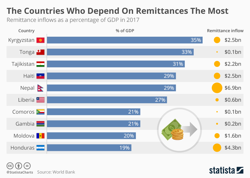
The population left behind may benefit from remittances of cash which the emigrants send back home, or money which they can earn as temporary foreign workers. Figure 20-0 shows that, for many countries, remittances are a significant source of income when compared to Gross Domestic Product (GDP). In 2018, remittances to low and middle income countries amounted to 526 billion US dollars[3], more than three times as high as official donations of foreign aid (149.3 billion dollars).[4].

The economy left behind may be hurt by emigration if the emigrants were better educated than average. This phenomenon is referred to as brain-drain. Canada is considered to suffer from brain-drain to the United States. Rural and remote communities suffer brain-drain to urban centres. The economy of the place of origin can also be hurt if it loses citizens who were harder-working, wealthier, or more politically active than average. Family and friends of emigrants will miss them.

If immigrants’ dreams come true, they will benefit from their move. However, many are disappointed by the limited opportunity to use their skills in the new country. Countries like Canada impose serious re-training requirements on teachers, doctors, and other professionals. Sometimes lack of language proficiency or discrimination are barriers to employment. Many immigrants pin their hopes for financial success on their children.
We shall see below that the citizens of the host country can materially benefit from immigration over the long term if immigrants bring skills, entrepreneurship, ideas and new technologies, and if it is easy to finance and organize new businesses.
A casual glance around the world shows that some of the most economically vital nations are nations which welcome immigrants and enjoy a great deal of cultural diversity.
Immigrants may be welcomed for their help supporting an aging population. The idea is that immigrants decrease the Aged Dependency Ratio and pay taxes that support social programs. Whether this is true depends on immigrants not having large numbers of dependents, and on immigrants providing a net fiscal benefit i.e. paying more in taxes than they consume in services.
In Canada, immigrants are immediately eligible for free language training, free health care, and public education. They use the existing infrastructure. After one year of residence they may apply for welfare and subsidized housing. Constantine Kapsalis (2021) estimated the net fiscal cost per recent[5] immigrant to be between $900 and $2,000 in 2015. While refugees and immigrants sponsored by family members were net recipients of government spending, Economic Class immigrants (representing the majority of immigrants) actually paid more in taxes than they used.
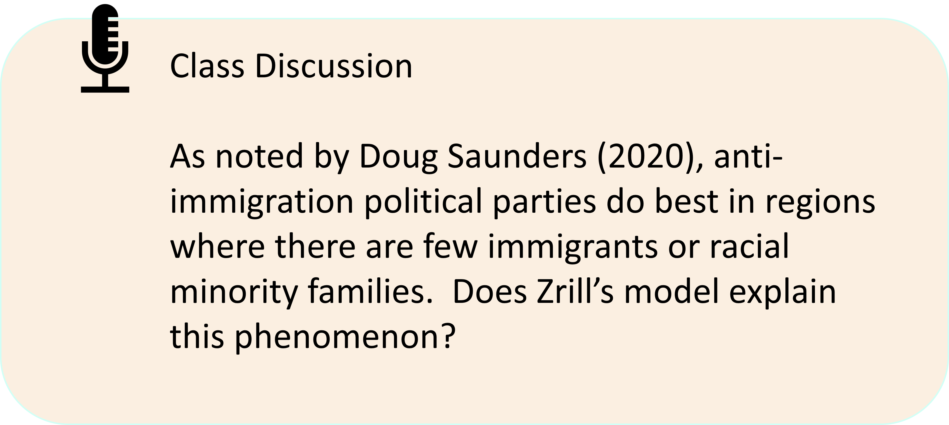
The host country may have concerns about immigrants’ ability and willingness to integrate. Zrill (2007) has a useful model of this.
Consequences of Immigration for Social Cohesion
In Zrill’s model, immigrants choose how closely to adopt the characteristics of native-born residents, whom we shall call “locals”. The more closely the immigrants conform to local customs, the more pleasant their interactions with locals will be, but the less pleasant will be their interactions with immigrants who have not conformed.
The more that residents, both immigrants and locals, resemble one another overall, the greater the community spirit or “social cohesion”. More social cohesion leads to more willingness to contribute to public goods[6], such as neighbourhood-watch programs, clean-up programs, community gardens, and local school programs.
Each immigrant chooses how much to conform to local customs, for example by choice of language, dress, and children’s names. This choice is modeled as maximizing a utility function which depends on the level of a public good as well as on the pleasure derived from the average encounter with another person. For each person encountered, the pleasure of the encounter depends on how similar the background characteristics of both people are, and on how similar the chosen characteristics of both people are. There is a tradeoff: the more an immigrant resembles local residents, the less awkward that immigrant feels meeting local residents but the more awkward they feel meeting immigrants who have not conformed.
Each immigrant and each local chooses how much to voluntarily contribute to a public good. In doing so they consider the utility the public good will bring to themselves and others. The utility of others is weighted: the higher the level of social cohesion, the more you care about other people’s utility. Thus, the higher the coefficient of social cohesion, the higher the supply of the public good will be.
Zrill works out a simple mathematical example where immigrants can only choose either to not conform at all or to conform completely. He solves for the tipping point between those two extreme choices. The tipping point is found at a particular ratio of immigrants to locals. If the number of immigrants becomes sufficiently high, no integration will take place. This is because encounters with other immigrants are relatively more frequent than encounters with locals, so conforming to other immigrants is more important than conforming to locals.
In Zrill’s model, the more ghettoized a group is, the more likely we are to get the non-integration, low public good case. While Zrill’s model intriguingly links customs, social cohesion, and public goods, it omits any benefits from cultural diversity.

Consequences of immigration for the standard of living
Setting aside consideration of social cohesion and public goods, we can use some simple math to uncover the direct material consequences of immigration for the standard of living.
As we saw in chapter 16, the standard of living, defined only in the simplest, most material way, can be broken down into three components:
Equation 16-1. Y/N = Y/H * H/L * L/N
Now we’ll condense the expression:
Equation 20-3. Y/N = Y/L * L/N
Where Y/N is output per person, Y/L is labour productivity multiplied by hours worked per worker i.e. labour productivity measured per worker instead of per hour, and L/N is the number of workers divided by the population. L/N is inversely correlated with the total dependency ratio, TDR.
When the population increases, either by natural increase or by immigration, the consequence for the standard of living depends on the impact of the population increase on labour productivity and on dependency.
To the degree that immigrants have few dependents and can find work, they will increase L/N.
If new immigrants receive more government services than they pay for, the distribution of GDP will be affected, but not necessarily GDP per person, unless the taxes used to pay for immigrants’ needs are negatively impacting labour productivity. From the native-born population’s point of view, however, net transfers of tax revenue to newcomers is a cost.
In this chapter we will call all people who are not newcomers “native-born”, for simplicity.
What about labour productivity? Does immigrant labour improve it? Labour productivity depends on efficiency and on the capital:labour ratio. Most people agree that a lot of immigrants are hard-working and that immigration improves efficiency. Immigrants arriving without money, skill, or new ideas, however, will drive down the capital:labour ratio K+/L, at least temporarily.
Consequences of immigration for the real wage
We noted in Chapter 18 that a growing population experiences a falling capital:labour ratio unless the savings rate is sufficiently high. We employed a constant-returns-to-scale aggregate production function, one example of which would be Y = A K+1/3L 2/3, where A is efficiency, otherwise known as “multifactor productivity”; L is raw labour, measured in person hours; and K+ is any kind of capital, including human capital like education, that workers can use. In this very macro model, there is only one good produced, so we can take the price of it as being equal to $1.
Dividing Y by L we see that labour productivity measured per worker is equal to Y/L = A (K+/L)1/3.
The expression for the wage is very similar. The wage is equal to the derivative of Y with respect to L, multiplied by the price of the output. Taking the price of output Y to be $1, the wage is equal to the derivative of Y with respect to L, which is 2/3 A(K+/L) 1/3.
Since this wage, reflecting what employers are willing to pay, is inversely related to L, we can draw the labour demand curve – the horizontal summation of individual employers’ demands for labour – as a downward sloping line in wage/person-hours space. A and K+ are held constant. It is graphed in Figure 20-1 below.

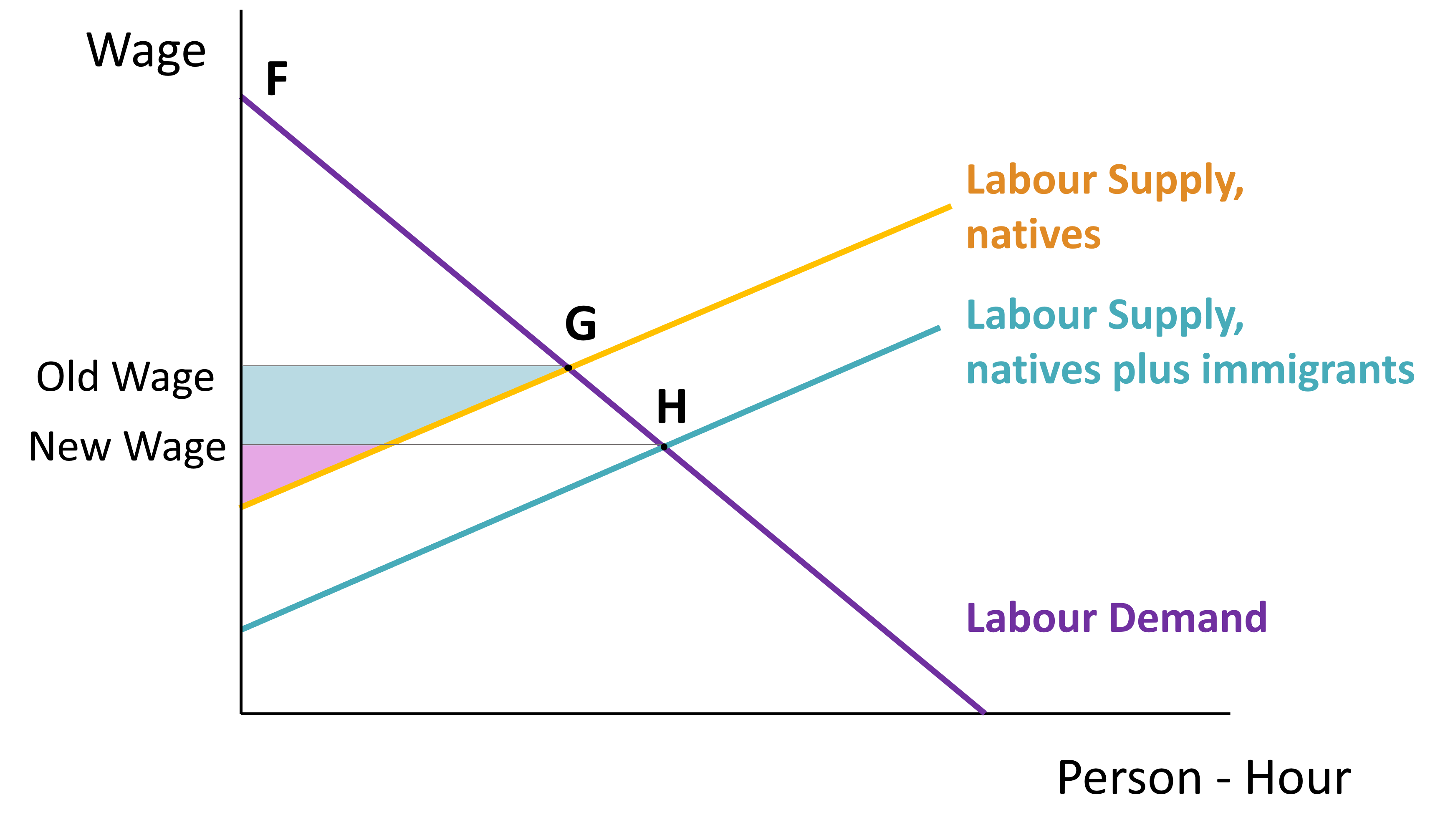
Since Labour Demand is a function of efficiency (A) and the capital:labour ratio (K+/L), any improvements in A or K+ will shift the Labour Demand curve to the right, resulting in higher employment.
This diagram is for a nation’s labour market as a whole. But it would be better to study labour supply and labour demand for particular occupations in particular regions. Not all occupations and regions will be equally affected by immigration.
Let’s examine Figure 20-1. Before immigration took place, the native-born workers earned the “old wage” and earned producer surplus equal to the light blue shape PLUS the purple triangle. This shows what native-born workers gain that is over-and-above their minimum requirements for compensation.
Once immigrants join the labour market, the wage falls to “new wage”. This is all about the capital:labour ratio dropping. The new wage line meets the native-born labour supply curve at a lower level of employment, indicating that some native-born workers are not willing to work at the new wage. Those who are willing earn a lower wage, and their producer surplus shrinks to just the purple triangle. So the light blue area is lost the native-born workers.
Figure 20-2 shows us who gains from an expanded labour market. Consumer surplus, which shows the difference between what employers would have paid (as shown by the demand curve) and what they had to pay (the going wage), has expanded. It has increased from triangle F-G-Old Wage to become F-H-New Wage. The increase is represented by the light blue shape (at native-born workers’ expense) and the bright blue triangle (pure gain). The immigrants earn the green area (pure gain), which is the area between the two supply curves and under the new wage.

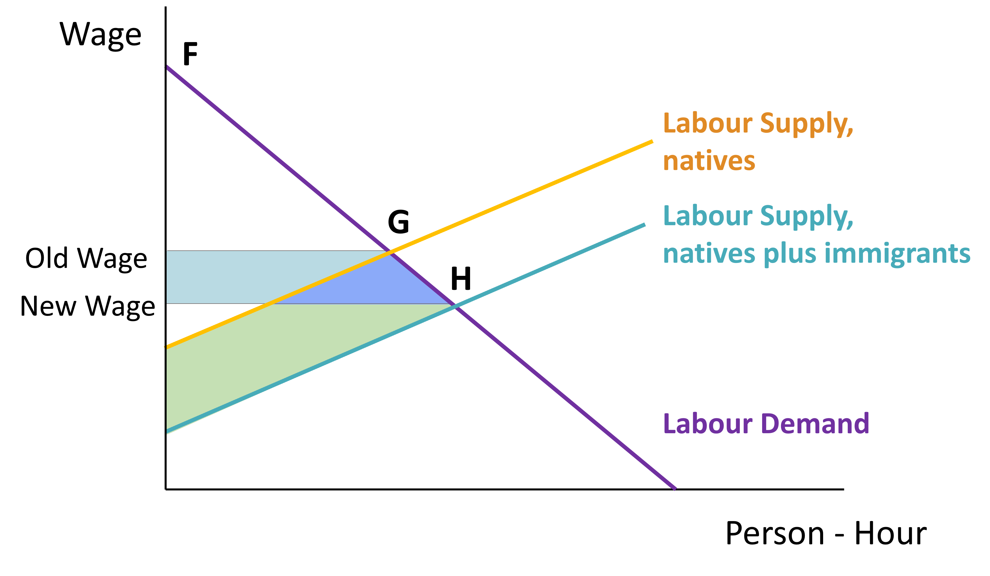
Comparing the total surplus (producer surplus plus consumer surplus) before and after immigration, there is a net gain of surplus equal to the green area plus the bright blue triangle. The bright blue triangle is the net gain to the host country’s population, and it accrues to employers, whereas the green area accrues to immigrants.
GDP has increased, but GDP per person may not have increased (yet)
GDP has increased because there is more of one of the inputs (labour); however, as we learned in chapter 16, GDP per person does not increase unless labour productivity improves or dependency falls. The material well-being of the average native-born person likely falls in the short run because their wage and labour force participation is reduced. They may also experience a redistribution of tax revenues from themselves to the immigrants.


Although an increase in the supply of raw labour depresses the wage, it is possible that the new workers bring with them some capital K+ or some new ideas A. If so, labour demand will rise and shift to the right, raising the wage.
Even if the new workers do not have any K+ or A with them, K+ can be accumulated over time through education or investment. The following factors will help speed the wage’s recovery:
- access to affordable education
- subsidies for research and innovation
- ease of starting new businesses: few regulations and fees.
- access to affordable loans
- ease of hiring and firing
In real life there is more than one production process and more than one labour market, and the price level is not equal to 1. The price level will be falling as lower wages in industries affected by immigration make for lower prices of goods and services produced in those industries. Workers may experience rising real wages if the cost of living is falling faster than the nominal wage pertaining to their occupation.
Table 20-1 summarizes what we have learned so far about the short-run effects of immigration on the standard of living.

Another short-run, likely persistent effect of immigration is that the population has grown larger. This can have both beneficial and harmful effects on the standard of living, as discussed in our previous chapter, Chapter 19.
In this Chapter we have learned that migration, both international and rural-to-urban, is very responsive to the expected real wage. Immigration into an area depresses the nominal wage of native-born workers until capital accumulation can catch up or until efficiency increases can give productivity a boost. Immigration increases the population’s size and diversity. It is likely to reduce the dependency ratio.
Having thoroughly explored the causes and consequences of voluntary migration, let’s see what Canada and the US have done and are doing with immigration. That will be the subject of Chapter 21.

- Complete the clear cells in the following table:
| July 1, 2009 | July 1, 2010 | July 1, ’09-July 1, ’10 | |
| Canadian population | 33,739,900 | 34,108,800 | |
| Change in population | |||
| Mid-year population | |||
| Births | 381,382 | ||
| Deaths | 247,556 | ||
| Natural Increase | |||
| Net Migration | |||
| Net Migration Rate | |||
| Migration Ratio |
2. If 40% of a nation’s population growth comes from net migration, what is its migration ratio?
3. In the life table for a nation, females have a 95 % chance of surviving until age 15, and males have a 94 % chance of surviving until age 15. 15 years ago there were 20,000 females born and 21,100 males. Today there are 19, 100 15 year-old females and 19,000 15 year-old males. Assuming no foul play, what is a rough estimation of the net migration of this cohort so far?
4. In the mid 1990s, universities and boards of education in Ontario offered generous early retirement packages. Who was most likely to take up such a package and “emigrate” out of the education system?
5. Wegge found that the villages that experienced the most emigration were those with that practised unigeniture (first son gets entire farm), and those that had higher emigration flows in the past, fewer factories, and more religious minorities. What is the relevance of each of these four factors to migration?
6. Describe an immigrant who poses least economic threat to a nation’s automobile assembly workers.
7. A large group of unskilled, poor, illiterate refugees arrives in your city. What can the city do to make sure that all residents benefit economically?
8. If a nation has a shortage of doctors, what are some ways of increasing the number of doctors?
9. Hanson (2007) estimated that for the United States, the bright blue triangle of lost labour market surplus for Americans was less than 0.07% of GDP, while the cost of patrolling the border was 0.1 % of GDP. Can he use these numbers to conclude that it does not make economic sense to patrol the border?
- Arends-Kuenning, Baylis, and Garduño-Rivera (2019) find this in Mexico, before and especially after implementation of the North American Free Trade Agreement. ↵
- "China's outdated residence permit system", UPI Asia.com, Feb 20, 2009, downloaded March 3, 2011. ↵
- Ratha et al (2019) ↵
- OECD (April 2019) ↵
- recent immigrants are here described as having arrived between 1995 and 2014. ↵
- A public good is a good which an entire community shares, and which does not diminish much with each use. Public radio programs, sewage plants, and public parks are examples of public goods. ↵
The real wage is the wage divided by a price index. The price index measures the cost of living. Thus your real wage measures the stuff you can buy for each hour worked.
The expected real wage is the probability-weighted sum of the different possible after-tax real wages or incomes you might receive in a particular location.
Remittances are monies earned by citizens of country x who work abroad temporarily, or gifts of cash to citizens of country x by those who no longer live in country x.
Brain-drain occurs when talented, wealthy, or otherwise useful citizens emigrate to another
community or another country
The word "fiscal" refers to government budgets. The net fiscal cost of an immigrant is the money the government spends on them and how much of the nation's shared infrastructure they use, minus the taxes the immigrant pays to the government.
Producer surplus is the benefit received by workers or sellers over,-and-above the minimum they require to provide the service or good. It is calculated as the difference between the wage received and the lowest acceptable wage, for the entire quantity supplied at that wage.
Consumer surplus is the amount by which the amount paid by buyers falls short of what they would have been willing to pay. It is measured as the area between the Demand curve and the price or wage.
