Now that we have considered the economic impact of the rate of population growth, let’s consider the economic impact of the population’s current size.

Even if the population is no longer growing, the population may be so large that just maintaining the population as its current size and standard of living requires the overexploitation of sensitive natural and environmental capital.  We see this possibility today as we face global warming due to human activity.  The level of carbon emissions rises with the number of people, other things being equal.  But other things may not be equal.  The level of carbon emissions also depends on production and consumption per person and the carbon intensity of that production and consumption.

carbon emissions = # people x carbon emissions per person

carbon emissions per person = goods consumed/produced per person x carbon intensity per good consumed/produced

That is why wealthier nations tend to have larger carbon footprints than poorer nations.  Canada in 2020 was the eleventh largest emitter of CO2 in the world, right after various Middle Eastern countries, and approximately thirty-ninth by population.

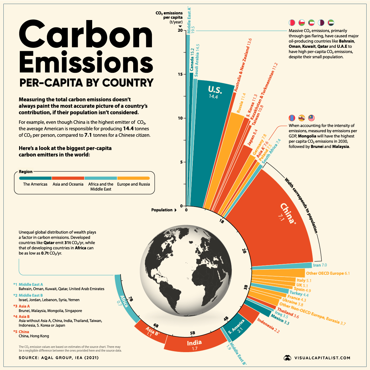
In Figure 19-0 above, the width of a country’s bar shows the number of people, and the height of the bar shows the carbon emissions per person.

We see that a population’s size is not tightly correlated to its carbon emissions per person.

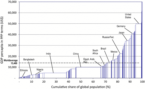
Figure 19-1 shows us data from 2011.  The width of the each bar indicates the size of the nation’s population as a fraction of the world population, while the height of the bar indicates its GDP per person, measured in US dollars and adjusted for differences in the cost of living.  Some of the largest countries are the poorest, but there are many exceptions.  The nation with the highest material standard of living, the United States, is not one of the smaller ones.

The next Figure compares per-capita income to population density for countries in 2020.  Both axes are in logarithmic scale because the differences measured linearly would be too great to fit all countries on the same graph.

Population density may be relevant to the standard of living inasmuch as capital – physical, environmental, social – may be strained within a particular region.  However, within a country, densely populated regions such as cities often feature more capital per worker than less densely populated regions.

Figure 19-2 shows us that, while many low-GDP-per-capita nations were densely populated in 2020, so too were the Netherlands, Singapore, and Hong Kong.

Consider that there are several ways in which population size and density can benefit a nation economically.  A large and densely populated nation potentially can enjoy more specialists, a thicker market, internal economies of scale, external economies of scale, and improved innovation.  Not that a small or sparsely populated country couldn’t enjoy some of these features.  If a small or sparsely populated country had extensive free trade relationships, a similar language and culture as its trading partners, excellent telecommunications and transportation networks, similar regulations, and few tariffs, national borders would be irrelevant and its small size would not matter.

Would you prefer to live in a larger city?  Would you prefer to attend a larger university?  Scale brings some advantages.

A larger population provides a greater variety of individuals, organizations, businesses, and educational institutions which, given opportunities, are able to make available specialized services and unique points of view.  To reap this reward, everyone should have equal access to supports and opportunities, and it should be easy to start new businesses.

When people are able to specialize, there are gains from trade as each person operates according to their comparative advantage.

In a dense population it is easier for buyers and sellers to find one another.  There is likely always something available in any product class.

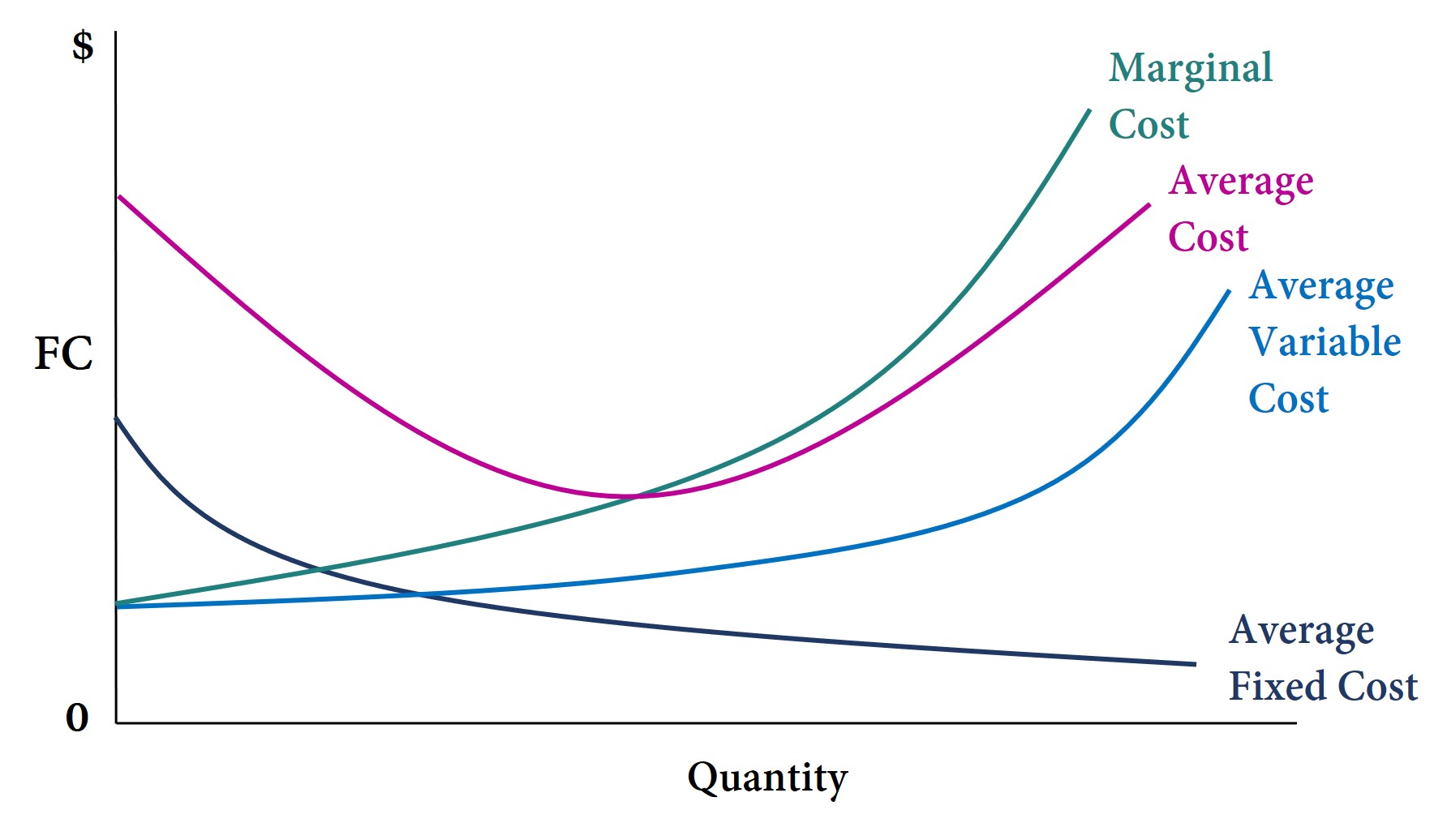
Businesses and governments spread fixed costs like buildings, advertising, and administration over the number of customers/citizens they serve.   The point at which average costs (the red line in Figure 19-3) are lowest is called an entity’s minimum efficient scale.

A business that has not yet reached its minimum efficient scale can achieve internal economies of scale by growing and increasing its output.  If the domestic market is very small, a firm might be able to achieve economies of scale by exporting; however, exporting entails complications like exchange rates, tariffs, and transportation across borders.

A business can also achieve lower costs by being near other, similar businesses.  For example, like a mini-Silicon Valley and a mini-Hollywood, Burnaby, British Columbia has attracted many film studios and tech companies.  For this reason, other film and tech firms are likely to locate nearby.  Together they will attract the talent, the attention, and the service industries they all require.  They may also become more productive by sparking off each other or by competing.  The profit a firm can earn by being part of a local industry is called external economies of scale.

Larger countries may have an innovation advantage.  For one thing, the research sector is likely larger.  This will support more specialists, and more internal and external economies of scale in research.

Another reason is that there is more economic activity in a larger country.  Some innovation develops spontaneously in a process of  learning-by-doing.

In addition to all the advantages listed above, there may be other material benefits of having a large population. For example, sheer size of population may be important, though not conclusive, militarily. Some groups desire population growth to ensure physical safety. Some groups desire a large population in order to preserve their unique culture, language, or beliefs.

Two prominent thinkers had very different ideas of whether population size would eventually overwhelm the natural world.  Julian Simon, an economist (pictured at left) and author of The Ultimate Resource (1981), argued that human ingenuity is the ultimate resource.  Human ingenuity will respond to scarcity with new ideas that permit more substitution for natural resources. Prices will signal scarcity and reward innovators. The standard of living can be sustained and improved with the help of new technology and new systems.

Paul R. Ehrlich (at right), a biologist and co-author of The Population Bomb (1968), argued that innovations buy only temporary respite from scarcity and mask the fact that we will not survive once natural capital is driven below a critical threshold. Our standard of living cannot be sustained, and it is jeopardized more and more by population growth.

In 1980, these two scholars made a bet about how high mineral prices would be in 1990. Simon was so sure that natural resources would not rise in price over the next decade that he allowed Ehrlich to choose any five resources that Ehrlich thought would become more expensive in real terms (i.e. excluding inflation). Ehrlich chose five different metals.  Each fell in price between 1980 and 1990, despite the world’s population having grown by 869 million people.

Not to be outdone, Ehrlich proposed a second bet. This time he wanted to wager that in 2004 compared to 1994 there would be less agricultural soil per person, less rice and wheat grown per person, lower sperm cell counts in human males, fewer plant and animal species in existence, a greater gap between the richest and poorest people, and so forth. This time Ehrlich was focusing on physical counts rather than dollar values.

Simon declined this new bet, saying it measured changes to human welfare only indirectly.

While we’re all hoping that world history will continue to back Simon’s point of view, there have been times when the sustainability of human culture and economic activity has been compromised by environmental degradation.

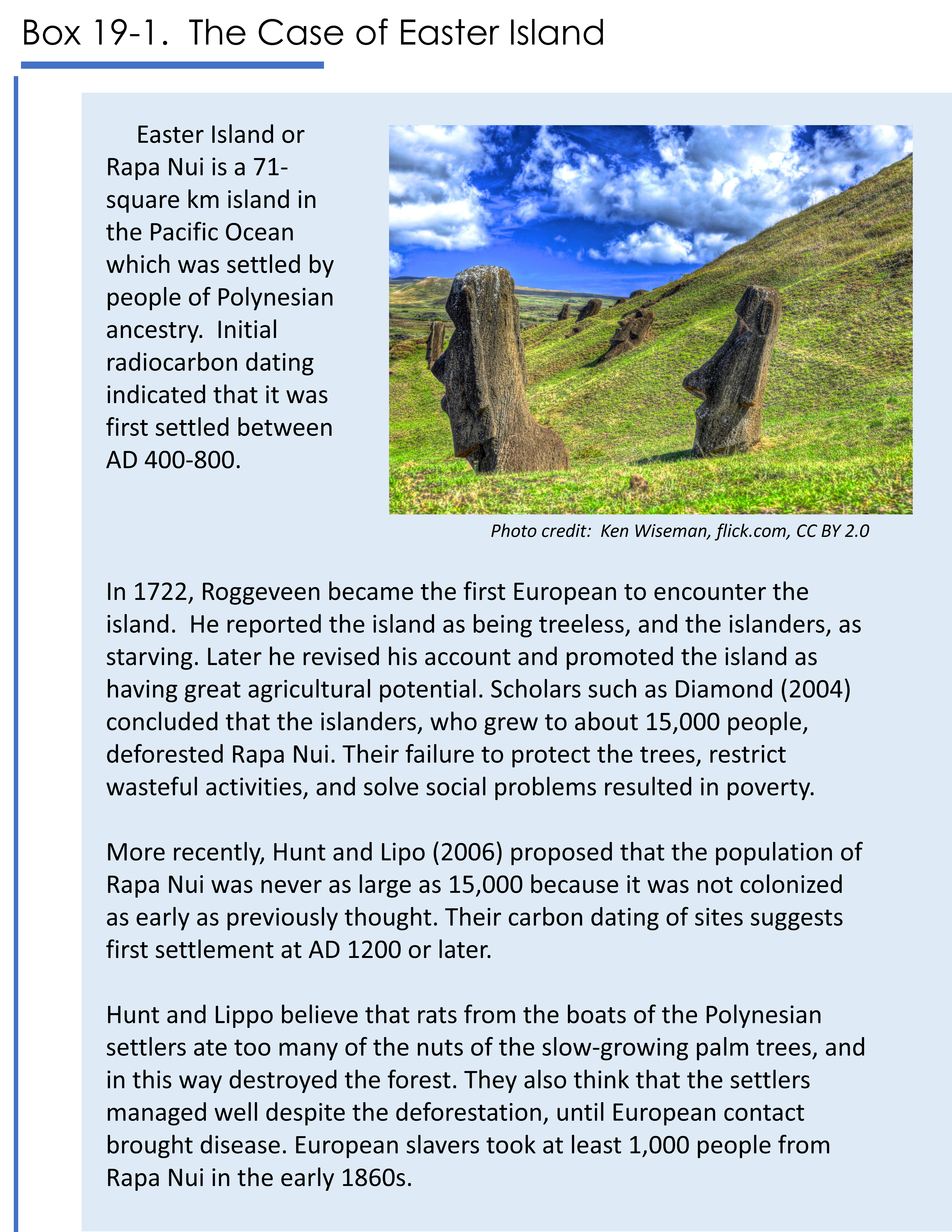
The case of Easter Island is the most famous example of environmental collapse.  But this case has recently been re-interpreted, as discussed in Box 19-1.

We will revisit the themes of sustainability and collapse in Chapter 25, as we summarize what we have learned in this course.  For now, we turn to study that third driver of population change, Migration.  Migration has the ability to change population size, density, and age structure in the blink of an eye.

1. Describe, as best you can, an actual place whose economy might benefit from a larger size population. Explain why a larger size population could be advantageous.
2. Give an example from real life where the internet is helping make markets
a) bigger
b) thicker
c) more friendly to innovation

3.  Replace this chapter’s “examples from the world of music” with examples from the world of football or soccer.