Governments usually exert some intentional influence on mortality, as well as on the two other drivers of population change, fertility and migration.  If effective, these policies may impact the every day lives of individuals and families profoundly.  The policies will also have an impact on the growth rate of the population, the eventual size of the population, and the age and ethnic composition of the population. The motivation of government may be economic or it may be based on values ranging from compassion to hatred.

What are the best practices around policy design?^[1]

Let’s begin with

1. No discrimination or coercion.  Can we agree that our government should work for the welfare of all ethnic and social classes, and all age groups? And can we agree that our government should not control our behaviour too closely?

Regarding coercion and control, it may not be easy to agree on exactly where the government crosses the line. For example, during the COVID-19 pandemic, a significant minority of people felt that the government had no right to mandate vaccination against COVID-19, and that employers, universities, airlines, and other entities had no right to require vaccination.

Regarding discrimination, during the COVID-19 pandemic in Canada and the United States, there were not enough vaccines, at first, to treat all who wanted to be vaccinated.  There were not enough hospital beds to treat all who were sick.  In terms of vaccine delivery, older adults, people with pre-existing conditions, and other vulnerable groups were prioritized.  But in terms of admission to hospital and care of the sick, it was the other way around.  In Canada, residents of long-term care facilities were often not taken to hospital.  The early, panic-stricken days of the pandemic saw many long-term care residents all but abandoned by staff.  In the United States, patients from long-term care were discharged from hospital back into long-term care facilities while still infectious and unwell.  Laura Appleman (2021) reports on this and also the inappropriate use of trial vaccines, even quack medications in long-term care facilities, as well as the neglect of psychiatric patients and people with developmental disabilities living in institutions.

Once we determine that a policy does not violate Human Rights, we examine the policy for its likely effectiveness, using the following guidelines:

2. Target the ultimate goal as closely as you can. Identify the ultimate goal or the root cause of the problem you are trying to address. Is the proposed policy the most direct way to achieve your ultimate goal? For example, perhaps the ultimate goal of the policy is to reduce deaths from COVID-19 virus, but the policy focuses on the sanitization of surfaces. Since surfaces are not a major conduit of COVID-19 transmission, this policy will not be very effective at reducing deaths from COVID-19.

3. Target the binding constraint. A successful policy addresses the most critical bottleneck, the most pressing barrier to achieving the goal or reducing the problem at hand. For example, if the policy is intended to encourage vaccination, you need to know what is really holding people back from deciding to be vaccinated. It will be no use offering free transportation to the vaccination clinic if people don’t want to go because they are afraid of the vaccine.

4. Target the appropriate margin. In microeconomics we learn that people evaluate things at the margin. They decide whether or not to study one more hour, not just whether or not to study at all. They decide whether and when to get the first shot of the vaccine, but then they also decide whether and when to get booster shots. Each margin needs to be considered.

5. Understand who pays the financial cost. Most people think that, if you tax consumers, consumers will end up paying more, and that if you tax firms, firms might be able to pass some of the cost onto consumers. This is partly correct. If you tax firms, they may or not be able to pass some of the cost onto consumers. Also, if you tax consumers, they may or may not be able to pass some of the cost onto firms. Therefore you cannot predict who will bear most of the tax unless you know the relative elasticities of Demand and Supply.

If Demand is very inelastic, and consumers are desperate for the product, they will pay the tax. But if they are not desperate, and can switch to other goods and services, they will refuse to pay more. Suppliers will end up reducing the price in order to keep their customers. Suppliers will end up receiving less than before, which means they have been taxed.  The least price-elastic party pays more of the tax.

In the case of a subsidy, we use the same logic. If a subsidy is applied to a product, people will want to buy more of it.  If Supply is very flexible, people will be able to go out and get as much of the product as they want, and they will enjoy the benefit of the subsidy. However, if Supply is limited, the increased Demand due to the subsidy drives up the price of the product. Consumers may not save much when they use their subsidy; instead, suppliers enjoy a higher price.  That means suppliers are benefiting from the subsidy. The least price-elastic party gains most of the subsidy.

 
Let’s look at an example.

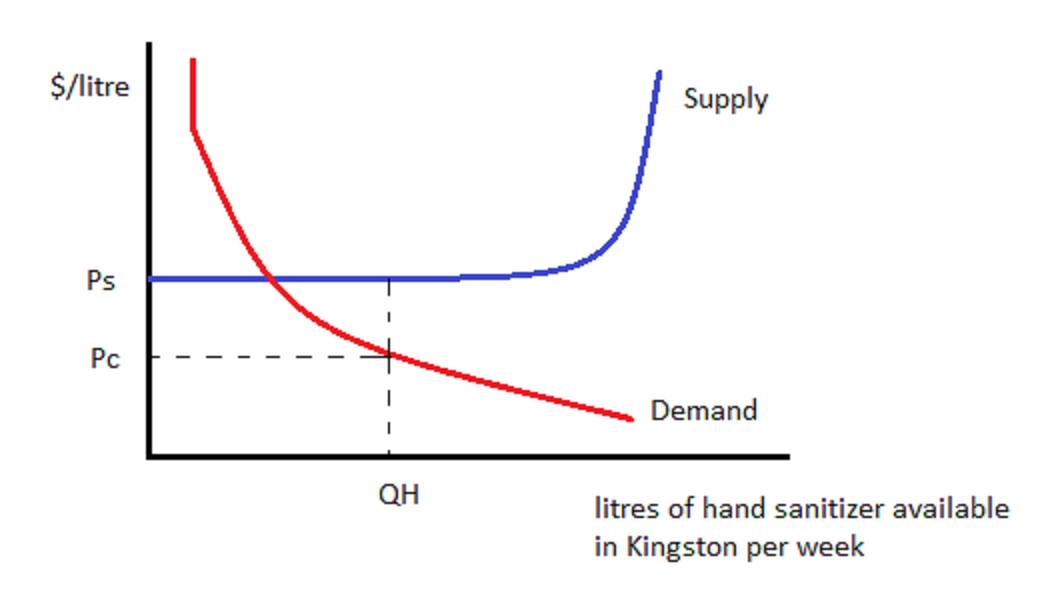
This graphic is a stylized depiction of  the market for hand sanitizer in Kingston each week before the pandemic. Because of Kingston’s hospitals, there is a very inelastic portion of the Demand curve, but after hospital demand has been satisfied, the rest of the Demand curve is not that steep. Meanwhile, there is enough hand sanitizer available to satisfy all of Kingston’s demand without affecting the going price of hand sanitizer.

Let’s label the market-clearing quantity of hand sanitizer in Kingston “Qm” litres per week. Let’s label the initial price “Pm”. Kingston is a small player in the hand sanitizer market and accepts the going price set by suppliers.

Now, what happens if, for some strange reason, the government were to impose enough of a tax on hand sanitizer to drive the quantity sold each week down to QL?

To get the Kingston market down to QL, the government imposes a tax per litre which is equivalent to the vertical distance between the two curves at QL, i.e Pc-Ps. We could draw the Demand curve shifting left until it intersects Supply at QL, or we could draw the Supply curve shifting left/moving higher until it intersects Demand at QL – it doesn’t matter. It doesn’t matter who is taxed – buyers or sellers!

In real life there may be some complications, but I’m going to keep things oversimplified to make the broader point – it often doesn’t matter who is taxed – buyers or sellers!

Whenever we draw a per-unit tax, we just have to move from Qm to the left until the distance between the initial Demand and initial Supply curves equals the tax, or until we get to the target quantity QL.

In this case, because the Supply curve is completely elastic, completely flexible, suppliers will not pay any of the tax. Instead, consumers will pay Ps + the tax = Pc. If you drew the Demand curve shifting left, you will see that consumer’s willingness to pay drops to Ps at QL, because they know they have to pay the tax on top of that.  The total amount paid is Pc, since the tax is equal to Pc-Ps.

The least price-sensitive party (Consumers) pay more (in this case, all) of the tax. Now let’s see that the least price-sensitive party (Consumers) get more of the subsidy.

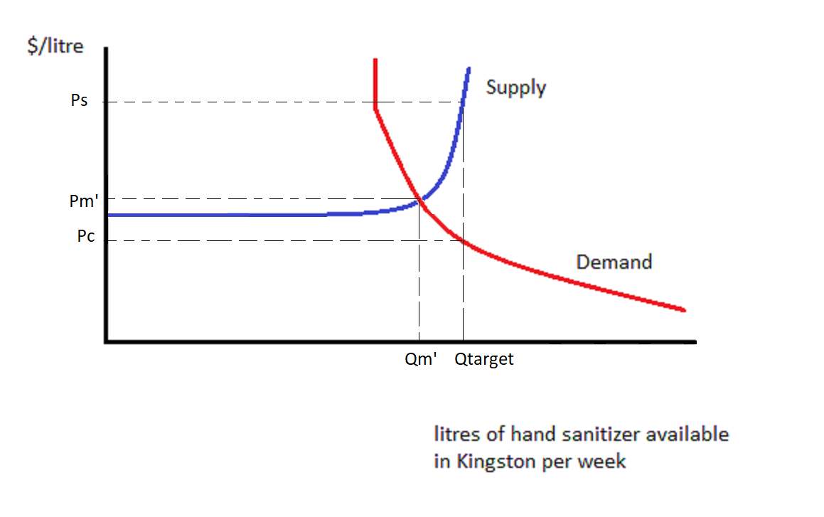
As we see in Figure 10-3, to draw a per-unit subsidy we don’t need to draw the Supply curve shifting to the right/down or the Demand curve shifting to the right. Either one would work, but it doesn’t actually matter which party is awarded the subsidy.

We move to the right of Qm until we get the targeted QH, which will occur when the vertical distance between the original Supply curve and the original Demand curve is equal to the amount of the subsidy.

Here we see that suppliers are receiving Ps as usual, but consumers are paying Pc which is below Ps by the full amount of the subsidy. If hand sanitizer subsidies were given to consumers, they would go out and buy more, but that would not affect the price of hand sanitizer, so consumers receive the entire benefit.

What if we were at the beginning of a pandemic, and Demand had shifted to the right a great deal, such that suppliers could not provide enough hand sanitizer without facing higher costs?  Let’s look at Figure 10-4.

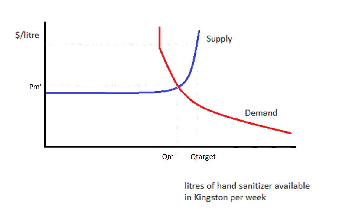
The market price has risen to Pm’, and quantity traded is Qm’.

Let’s explore what happens if the government subsidizes hand sanitizer to the point where Qtarget litres of hand sanitizer are purchased each week.  That can be shown by drawing a vertical line at Qtarget.  It’s not necessary to ask whether consumers or suppliers are receiving the subsidy.  We could draw Demand shifting to the right until it meets Supply at Qtarget, or we could draw Supply shifting to the right/down until it meets Demand at Qtarget: the result is the same.

What we see is that, at Qtarget, consumers are paying Pc which is a bit less than Pm’.  Suppliers are receiving Ps which is a lot more than Pm’.  Each of them is doing better than they would do if there were no subsidy.  They are sharing the subsidy.   Suppliers are receiving a larger share of the subsidy due to the Supply curve being less elastic than that of the Demand curve at Qm’.  It is more difficult for Suppliers to respond to price than it is for Consumers.

To sum up, policies designed to help consumers may help firms more, if supply is inelastic.  The inelastic party benefits more from a subsidy.  The government might subsidize milk in order to get consumers to drink more milk.  But if the supply of milk is inelastic, milk suppliers will raise the price and capture most of the benefit of the subsidy.

Similarly, the inelastic party is hurt more by a tax.  A tax designed to curb consumer behaviour may have more of a financial impact on firms instead, if supply is inelastic relative to demand.  An example of this might be a tax on sugary beverages.  If consumers are happy to switch to sugar-free drinks, the suppliers of sugary beverages will have to lower their prices by almost the entire amount of the tax, so that the tax-inclusive price is not much different from the original price.  The good news is that at this lower price, fewer sugary drinks will be supplied.

We have learned how to design good policies.  They respect human rights.  They are also well-targeted and effective, so they are likely to have a high ratio of benefits to costs.  We may wish to formally evaluate a policy or project by comparing its benefits to its costs.  When the project saves lives or prevents sickness and injury, we quantify the health-adjusted life years saved (HALYs), also known as quality-adjusted life years (QALYs).

For each person saved from death, their life years remaining are credited as benefits of the project.  The life years remaining to a person saved depends on that person’s age at the time the policy or project was implemented.  Thus projects that save young lives will be regarded as more beneficial than projects that save older people’s lives.   Each year of life remaining may be scored between zero and 1, or conceivably even less than zero, according to how healthy and able that person is expected to be.  (The same procedure of scoring health is used to form the Health-Adjusted Life Expectancy, discussed in Chapter 6.)  The health scores for different illnesses and disabilities are based on interviews.

For each person saved from disease or injury, we add up their life years saved, scored for health.  So we add up all the life years added to people’s lives because of the policy or project, adjusted for health.

Having quantified the saving of life, do we need to affix a price to each HALY saved?
&nbsp?;
If we use Cost Effectiveness Analysis, we can avoid pricing HALYs.  Instead, we will calculate the net cost of the project per HALY saved.  The number of HALYs saved will be in the denominator, and in the numerator we will put the sum of all project costs minus the sum of all project benefits other than HALYs saved.  The costs and benefits in the numerator will be measured in dollars according to their present value.

In Figure 10-6 we see a HALY/QALY supply curve for a hospital.  The hospital can save lives and prevent disease and disabilities by implementing a variety of projects, be they policies, treatments, or other plans.  Their first choice will be to spend as much money as they can afford on project A, which has the lowest net cost per HALY.  We see the cost per HALY rising a bit over the course of project A, perhaps because it begins to be applied to people who are less amenable to its treatment.  After project A cannot be expanded any further, or becomes too expensive, the hospital switches to project B.

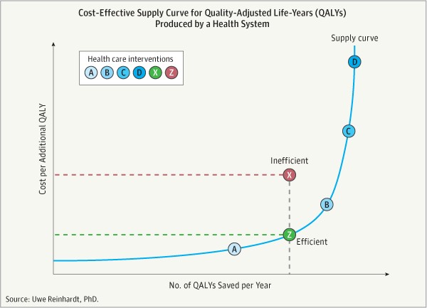
Using Cost Effectiveness Analysis in this way is appropriate when the paramount goal of the planner is to save HALYs.  When other benefits are important, Cost Benefit Analysis is more appropriate.

For Cost Benefit Analysis, we must price all the benefits (in dollars, present value) and subtract off all the costs (in dollars, present value.)  This means that we have to find a dollar value for a HALY.

Remember that, in the Life Table, we calculate the deaths of an initial cohort of newborns at each stage of life.  At each stage of life, we don’t know which newborns will die.  We only know what fraction of newborns will die.  That’s our lived experience.  We don’t know if we’re going to get hit by a car if we jay-walk; we just know the odds.  We don’t know if we will experience a workplace accident; we just have a rough idea of the odds.

If we were to to accept an increased risk of dying on the job, say an increase of 1 in 100,000 chance of dying, in exchange for one extra cent of wages per hour, then that means that for $0.01 x 2,000 hours per year =$20 per person, multiplied by 100,000 people (of whom one will die), we have accepted $2,000,000.  We have accepted $2,000,000 for one statistical death.  This is the “Value of a Statistical Life” (VSL).  Economists and others have estimated the VSL after statistically teasing apart wages by occupation, education, experience, risk of accident, and other factors.

This may seem a very crass exercise indeed.  But do we not, in a way, make this calculation every time we take a risk walking or driving or eating junk food?

We should never interpret the VSL as permitting us to kill someone for that price.  We would spend much more than the VSL saving the life of someone known to be in trouble e.g. a child fallen down into a well.  We only use the VSL to put a price tag on an increased chance of dying or to put a dollar value on an anonymous life year possibly saved.

The VSL represents the sum of the present value of each of a person’s life years remaining.  Thus having estimated the VSL for people age 40, who typically have 36 HALYs remaining, say, we could compute the value of a HALY from the perspective of people age 40.  The VSL for older people will necessarily be less than the VSL for younger people, ceteris paribus, because younger people have more expected life years remaining.

It’s tough to deal with the fact that some life-saving treatments and projects will be rejected by Cost Benefit Analysis as being too expensive.  But it’s good to know that there may be more affordable ways to save lives, as identified by Cost Effectiveness Analysis.  We can craft our policies wisely and organize our spending efficiently to save as many lives as possible.

1. In order to reduce mortality rates, the Canadian government decides to send Canadians a rebate of $50 per bicycle purchased. Analyze the incidence of this subsidy. Analyze the likely effectiveness of this subsidy at reducing mortality rates in Canada.

2. Under what conditions will heightened COVID-19 safety protocols increase the price of food at burger chain restaurants?