In our previous two chapters we explored how the age structure of the population affects the economy.  Now we focus on how the rate of population growth affects the economy.

The model of economic growth by Robert Solow (1956) is very well-known, simple, and easy to manipulate, so we’ll have a look at it and see what it predicts about the economic consequences of  population growth.  Its message will not be about efficiency, because efficiency is held constant in the Solow model.  It will not be about hours worked or about the fraction of the population that works, because in the Solow model, labour is measured as the number of people in the population: everyone is assumed to work full-time.

The Solow model’s message will be about the capital-labour ratio, K/L, and the importance of accumulating capital to keep up with the number of workers.

The Solow model uses the aggregate production function Y = A F(K,L)

Y = aggregate output of the economy.  There’s just one thing produced.

A = efficiency.  This is held constant.

F(K,L) = the production function.  The production function exhibits constant returns to scale; that is to say, if you double K and double L, F(K,L) doubles in size.

K = physical capital.  This time we are not using K+ as we did in Chapter 16.  K+ represents a number of different kinds of capital, and different kinds of capital may present mathematical complications.  For example, if we include human capital, we might reasonably expect that human capital accumulation would affect efficiency, A, and we’d need an equation to show how that happens.  If we included non-renewable natural resource capital, we’d need an equation to show how the resource stock is being depleted.

L = labour.  This is identical to the number of people in the population.  It grows at rate n.

Why is efficiency A held constant?  We might think of including an equation that shows how efficiency grows, either exogenously (automatically) or endogenously (in response to something in the model, such as population growth).  However, if A is allowed to grow, then output Y exhibits increasing returns to scale.  Doubling K and L while increasing A would result in more than double the output.  If increasing returns to scale were in place, output Y and consumption could grow forever in the presence of population growth.  Sustainability would be too easy, at least mathematically.

Because efficiency growth such as technological change makes sustainability so easily to achieve, it’s more interesting to hold technological change constant and see what happens when technology and other forms of efficiency don’t improve.

We think of efficiency A as possibly changing depending on the age structure of the workforce, but in the Solow Model there is no change to the age structure.

This model is almost as simple as the Malthusian model.  One difference is that in Solow’s model the population growth rate never changes.  A second difference is that in Solow’s model, there is not only labour, but also physical capital.  People can either eat the output Y or save some of it.  The saved Y is invested and is transformed into capital.  Think of Y as corn, which you can either eat or save for planting next spring.

The production function F(K,L) can be any positive monotonic function of K and L so long as

• Both K and  L are essential to production.  If one of them is equal to zero, then output must be equal to zero.
• There is some degree of substitutability between K and L.
• F(K,L) demonstrates diminishing marginal returns to K and to L.
• F(K,L) exhibits constant returns to scale.  As noted above, if you double the inputs, you double the output.  Similarly, if you divide the inputs by some number, you divide the output by that same number.  This makes it possible easily to express the production function in terms of output per worker, dividing by L.

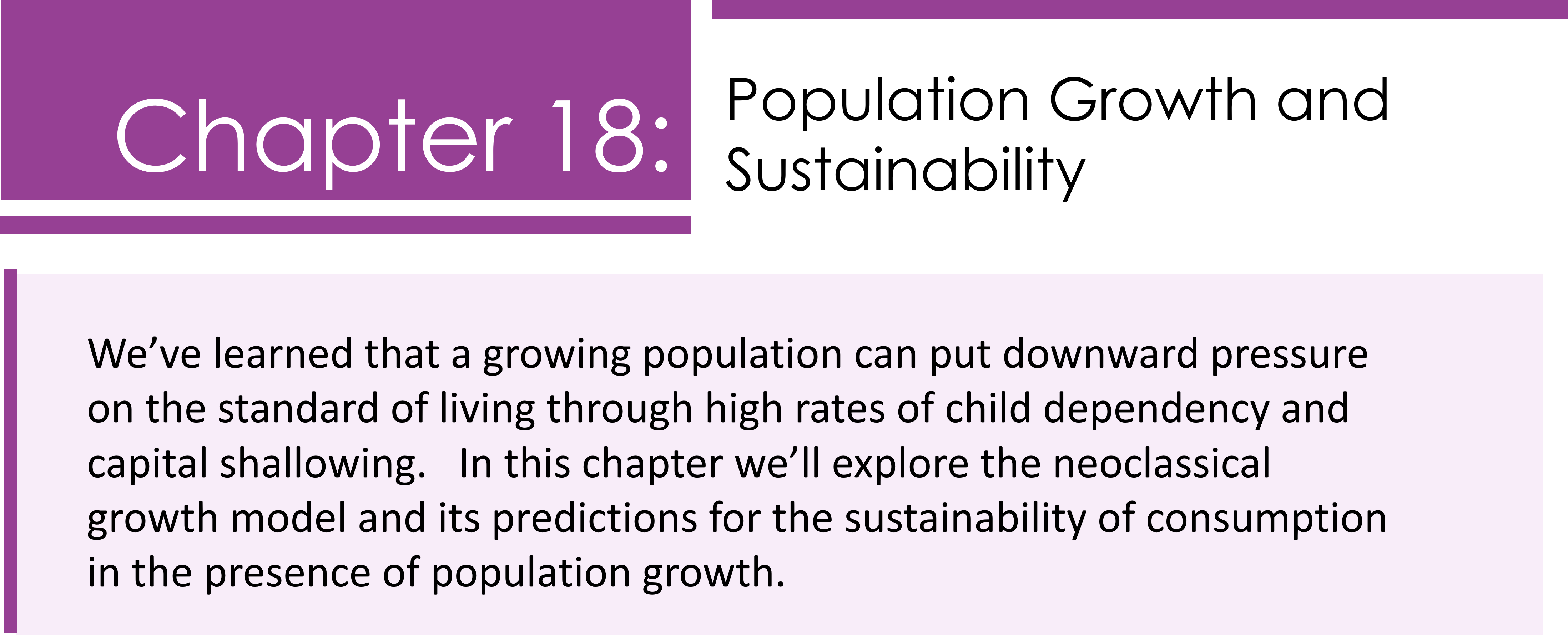
Assuming constant returns to scale, Solow divides everything by the number of workers so that there is one production process y=f(k) which uses capital-per-worker k to produce output-per-worker y.  Capital-per-worker is denoted by lowercase k and is called the capital-to-labour ratio or capital:labour ratio.

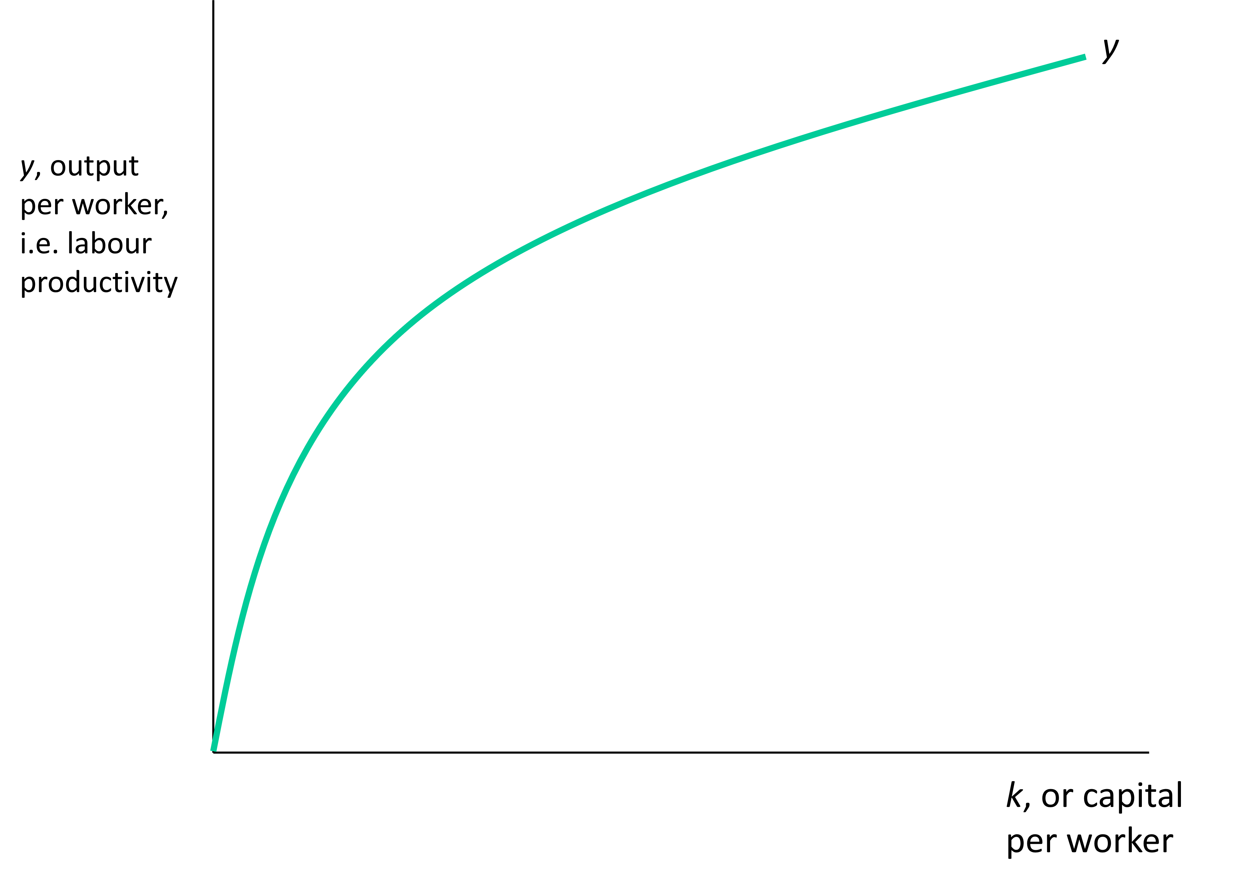
Figure 18-1 shows output-per-worker as a function of the capital:labour ratio.  This function demonstrates diminishing marginal returns to k.

Figure 18-2 shows the same function multiplied by fraction s.  s is the savings rate.

In the Solow model, we produce y, which represents output per worker or output per person (since all people work).  Fraction (1-s) of this is consumed, and fraction s is saved/invested into the stock of physical capital, K.  Every year, K increases by sY.  It can be shown (if interested, see the end of this chapter) that the amount of savings needed to keep the capital:labour ratio steady must satisfy Equation 18-1.

The amount saved per worker must equal the population growth rate/labour force growth rate multiplied by the capital:labour ratio.

The original Solow model also included another term, called d.  d is the rate at which physical capital depreciates, by rusting away or becoming obsolete.  If you include d in the model, Equation 18-1 becomes sy=(n+d)k.  We show that at the end of this chapter.

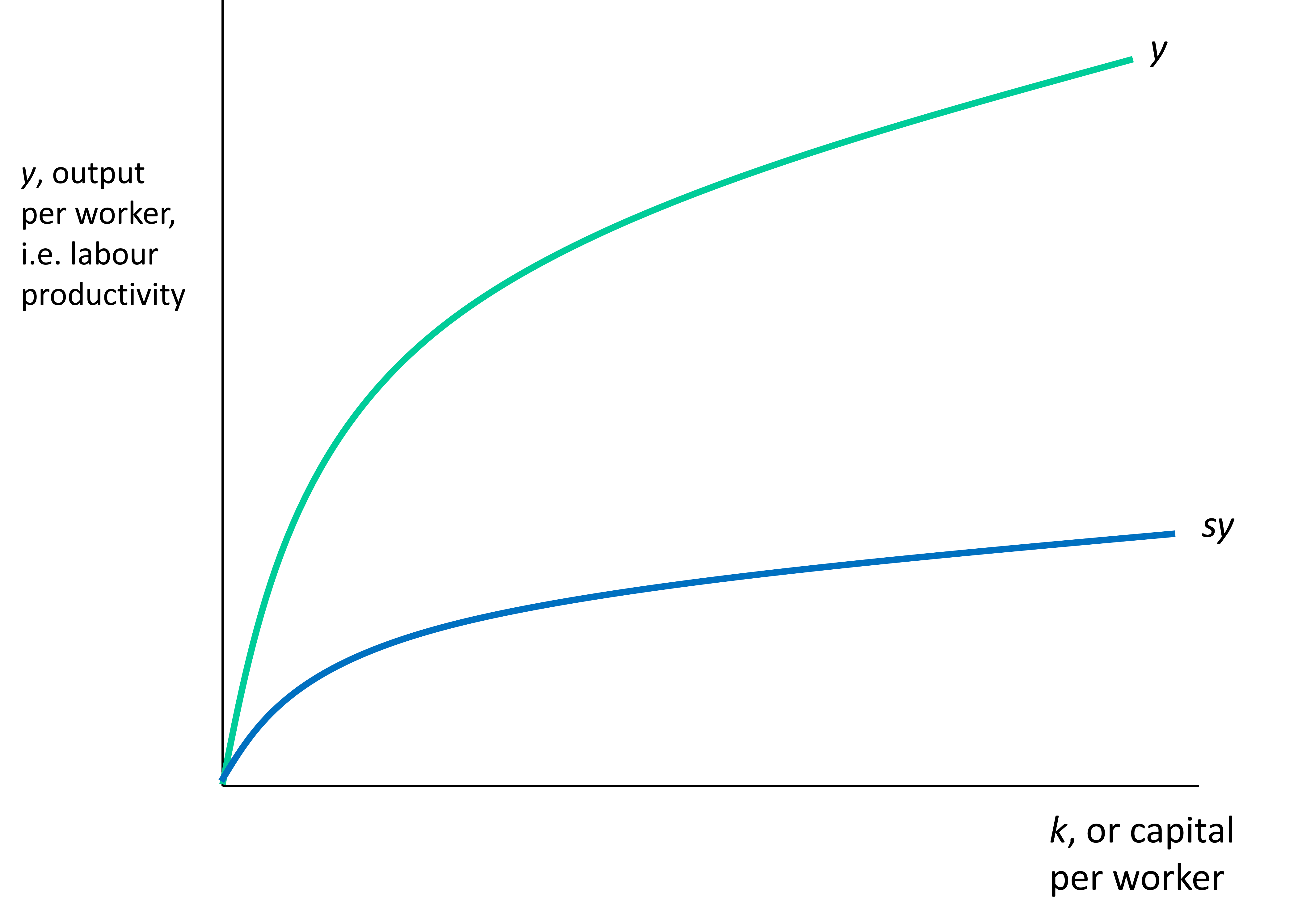
According to Equation 18-1, sustainability requires that a population must save enough to offset something, something to do with population growth.  Let’s have a look at Figure 18-3 to learn more.

The blue line above, sy, represents the left-hand side of the Solow condition (Equation 18-1), while the yellow line, nk, represents the right-hand side.  Where these lines intersect is the level of k, where the Solow condition is satisfied.

The lines intersect at a particular level of k, called the steady state capital:labour ratio, or k*.

Wherever the blue savings line is higher than the yellow population line, sy > nk, and the capital:labour ratio rises.  As it rises, we move rightward along the horizontal axis until we get to k*.

Wherever the blue savings line is lower than the yellow population line, sy < nk, and the capital:labour ratio falls. We call this “capital shallowing“.  As k falls, we move leftward along the horizontal axis until we get to k*.

So whatever capital:labour ratio k we start out with, we tend to reach k*.  k* is an equilibrium.

If we start out with a k that is higher than k*, k falls.  That’s because k is so high that diminishing returns are kicking in, and the extra output we get from our investment is not enough to prevent capital shallowing.  If we start off with a low k, we will find that our savings and investments are so productive that capital accumulates faster than population.

This is exciting! Whatever savings rate we choose, we can achieve:

Even though the labour force in the Solow model is constantly growing at rate n, the amount each worker/person consumes will never fall.  Consumption per person never falls = that’s what theoretical macroeconomists call sustainability.  Like a lot in economics, the conception of sustainability is very anthropocentric.

Population growth will cause capital shallowing, but we can save and reverse that capital shallowing.  By means of saving, the capital stock can grow as quickly as the population.

If the population growth rate were to rise for some reason, our yellow population line would become steeper.  It would intersect the blue savings line at a lower k*.  This would means lower output per worker and lower consumption per worker.  However, the output and consumption per worker are still constant every year.  They are still sustainable.  Consumption may be reduced because population growth has accelerated, but it is still sustainable, unless it falls below the critical threshold needed to support human life.

If the efficiency level A were to rise for some reason, again our blue savings line would pivot up and intersect the yellow population line at a higher steady state k*.  Output per worker would rise, and so would consumption per worker, since output has increased and the savings rate has not changed.

If the savings rate were to increase for some reason, our blue savings line would pivot up and intersect the yellow population line at a higher steady state k*.  This would result in a higher steady state level of output per person; however, because a higher fraction of that output is being saved, it’s not clear whether consumption per person would actually increase.

We can solve mathematically for the savings rate that would result in the highest level of consumption per person.  That savings rate is the one that achieves the “golden rule” k*.  The golden rule k* is found where the slope of the per-worker production function (y=Y/L=Af(k*)) is equal to n.^[1]

The Solow model tells us that, if we save, we can achieve sustainability of consumption despite population growth, unless the rate of population growth is so very high that k* and the resulting consumption  (=(1-s)y) are too low to support life.  In the real world, things are more complicated. The Solow model ignores the natural environment.  It ignores the fact that not everyone works.  And it assumes that the rate of population growth doesn’t affect how much people save.  In the real world there is environmental degradation, there is dependency, and there is the likelihood that dependency reduces workers’ savings.

When the rate of population growth is increasing, it is likely that the young dependency ratio (YDR) and total dependency ratio (TDR) are increasing.  It is likely that savings will fall as parents devote resources to caring for the young. Kelley (1998) calls this the youth dependency effect. It is also likely that governments will spend on education and health care for the young, diverting money away from investment in various forms of physical and knowledge capital.  Most of the spending on children will not improve the productivity of the current working generation. Kelley calls this the investment-diversion effect.

A. C. Kelley (1998) reviewed the many journal articles on population and economic growth available at that time.  He concluded that, ceteris paribus, the rate of population growth likely reduces the standard of living through the youth dependency effect, the investment-diversion effect, and capital shallowing.  However, there is no clear empirical relationship between the population growth rate and per capita output. Many other important factors also influence per capita output, factors like the economy’s overall size, its civil and political institutions, its educational achievement, and its openness to trade (Bloom 2003).

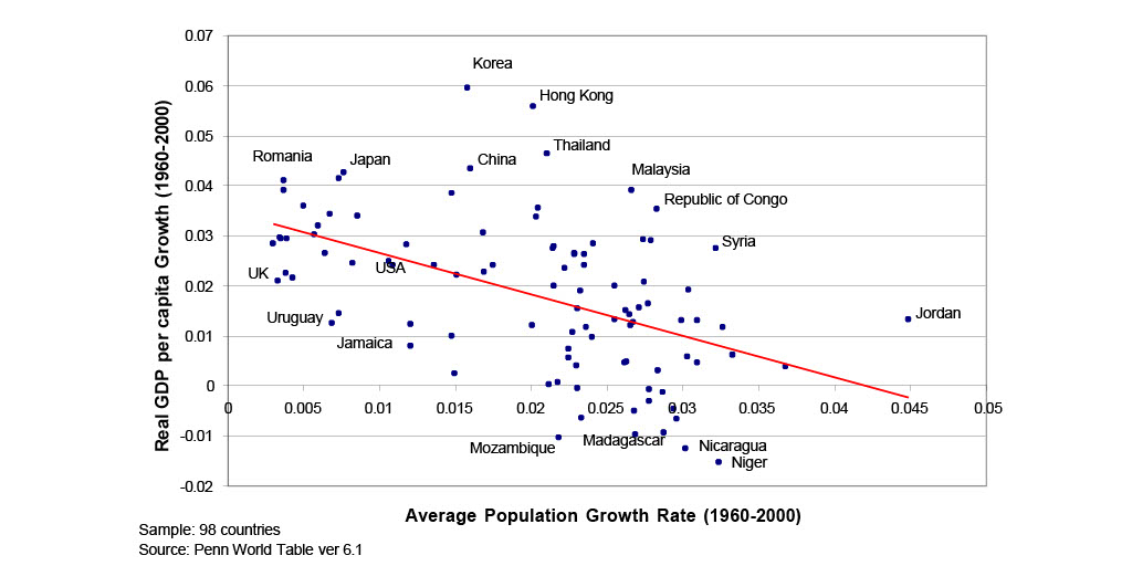
If we observe an apparent negative correlation between income growth and population growth, we have to remember that causation can flow both ways in a negative feedback loop.  Low economic growth could mean lower rates of female education, low rates of female employment, higher rates of infant mortality, and a smaller social safety net, all of which tend to increase fertility.

The graph below shows GDP per capita growth, adjusted for inflation, between 1960 and 2000, for 98 different countries, as a function of the average population growth rate for each country between 1960 and 2000.  A simple best fit line has been generated.   Variation in population growth rates “explains” 25% of the variation in GDP per capita growth, or vice versa.  75% of the variation remains unexplained.

The Solow model paints a scenario where saving prevents consumption per worker from falling as the population grows.  Could that work if there are natural resources needed for production?

The Solow model will continue to generate sustainable output and consumption per worker when the production function includes a renewable resource.  The renewable resource must be harvested sustainably.  No more of the resource each year can be harvested than can grow back in one year.  In fact, we should harvest less than that, because the stock must continue to grow as long as population grows.

When we add a non-renewable resource, such as oil, coal, or lithium to the production function, the Solow model can no longer generate sustainable output or sustainable consumption in the presence of population growth, at least not as long as population growth is geometric or exponential.

In the Solow model, savings can compensate for capital shallowing and capital depreciation, or savings can compensate for non-renewable resource depletion, but not both.

If there were no population growth (i.e. n=0) and no depreciation of capital (i.e. d=0),  then consumption could be sustained despite the depletion of non-renewables like oil.  Solow (1974) and Hartwick (1977) showed that IF physical capital can substitute to some degree for non-renewables like oil, and IF enough physical capital were accumulated to make up for the diminishing stock, then consumption could be sustained indefinitely.

Hartwick derived the formula for the precise amount of savings needed to make up for declining non-renewable resource stocks. The amount needed is equal to the amount of non-renewable resource extracted multiplied by rent (price minus marginal cost) on the marginal ton. This amount is known as Total Hotelling Rent.

Hartwick’s Rule tells us to invest non-renewable resource rents in other forms of capital.  This will keep our output and consumption steady, so long as the savings rate is not affected and dependency is not an issue.  If there is geometric or exponential population growth, sustainability is not achievable; however, if there is arithmetic or quasi-arithmetic population growth^[2], sustainability can be achieved by investing even more than Total Hotelling Rent.

In real life, our population has grown and our capital stock has more than kept up, because of technological improvements, other efficiency improvements, and the colonization of new lands and peoples. Neither Malthus nor Solow nor Hartwick include technological change in their models.  That is because the introduction of technical change into a mathematical model will too easily generate sustainability.

Hartwick’s Rule depends on the production function being the kind where the inputs are multiplied together to yield the output. This means that it is always possible to make up for a shrinking amount of one input by using more of another input. In Hartwick’s model, an expanding stock of K makes up for a diminishing stock of non-renewable resource.   R. Herman Daly (1990), one of the founders of Ecological Economics, has pointed out that there may be critical thresholds below which all the physical capital in the world cannot make up for the loss of natural or environmental capital.

Ecological Economics was established as a discipline in 1990 by economists who were concerned that traditional economics does not adequately consider the economy’s size and the population’s size relative to the carrying capacity of the environment.  We will discuss population size in our next Chapter.

We can take Hartwick’s Rule as suggestive rather than definitive. It recommends something that common sense immediately recognizes: do not allow the stock of your capital to diminish. Invest the profits you earn from nonrenewable resources. Save for the day when your resources run out.

Many nations have created sovereign wealth funds to invest the tax revenue that their governments collect from the oil and gas industry.  Alaska, Kuwait, and Norway have such sovereign wealth funds.  Alberta contributed to its Sovereign Heritage Savings Trust Fund between 1976-1988, and 2005-8, but otherwise the revenue has been used by the government or distributed among Alberta’s residents. Chile and Venezuela use resource tax revenues to help with government spending needs.

Genuine Savings, also known as Adjusted Net Savings, is an estimate of whether a nation’s capital stock (including physical, human, natural, and environmental capital) is really growing or not. If genuine savings is positive, then the nation is wisely building up its capital stock. If genuine savings is negative, then the nation is dissipating its capital.

Here is the calculation:

If the rate of genuine savings is positive, the nation is accumulating capital.  The question then is whether the rate of capital accumulation is high enough to match population growth.

In Table 18-1 we see estimates of Genuine Savings (as a rate) for several countries, computed by the World Bank.

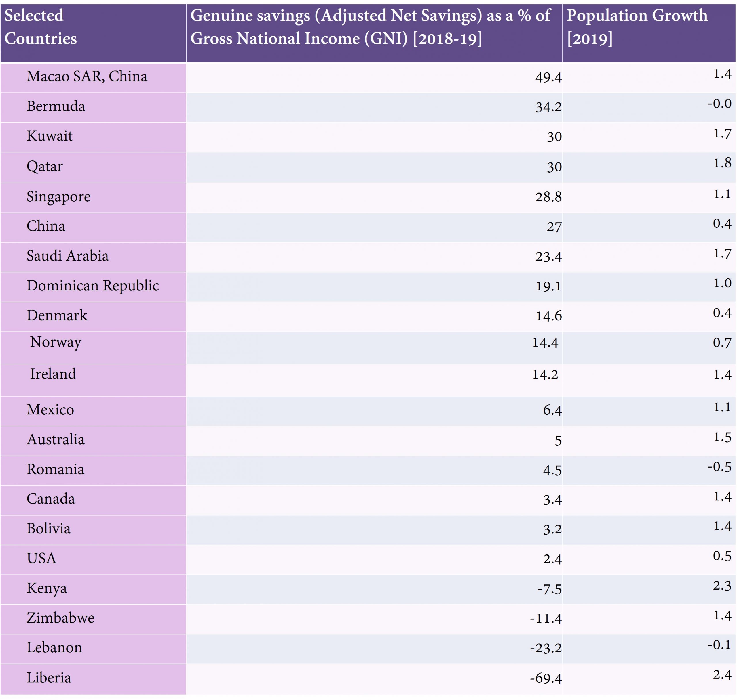
[58] Compiled by Pauline Galoustian.  Sources: World Bank (data.worldbank.org) /United Nations Population Division/Eurostat: Demographic Statistics/United Nations Statistical Division/Secretariat of the Pacific Community (CC BY 4.0)

How can we tell whether the Genuine Savings of a country is enough to keep its consumption sustainable?  If the population is not growing, any genuine savings above zero indicates an increase in the productive capacity of the economy and an improvement in its ability to provide consumption sustainably into the future.  If the population is growing geometrically or exponentially (as is usually the case), then Genuine Savings needs to be impossibly high unless technical change and efficiency improvements are occurring (as is usually the case).  In the situation of population growth with technical change, we don’t have a simple equation to calculate how high a nation’s Genuine Savings needs to be.

The World Bank (2011), in its Appendix E, tried to estimate that anyway.  Their calculations for the year 2005 purported to show that Canada’s genuine savings that year had been sufficient to cover its population growth.  They also estimated that the United States had needed to save an additional 2% of gross national income in 2005 to keep its capital-per-person (they did not calculate it per worker) intact.

In our next chapter, we’ll study the effects on the economy of the absolute size of the population.

The end-of-chapter questions follow the Appendix below.

Let K(t) be the capital stock at time t.  s is the savings rate. d is the rate at which capital breaks down or becomes obsolete: the depreciation rate. We will set d = 0 for simplicity.  L(t), the labour force at time t, is growing every year at rate n.

The production function is:

A(t) is efficiency or technology at time t and we just hold it constant, meaning:

Dividing by L(t), we write y(t) = A f (1, k(t))  where y is output per worker and k is capital per worker.

We can ignore the 1 and write:

The following equation shows how the capital stock grows from year to year:

Translation: capital next year = capital this year + amount saved minus capital lost to decay and obsolescence. Rearranging:

What we’re going to do now is divide everything by K(t).

Using the fact that,

the equation becomes:

The left-hand side is “percentage change in K”. Now the percentage change in little k is equal (by definition) to the percentage change in K minus the percentage change in L.  The percentage change in L is the population growth rate, since in this model, everyone is in the labour force. So let’s replace the left-hand side of our Solow equation with the percentage change in k plus n, the population growth rate.

Now multiply both sides by k(t) and we have our final version:

This is Equation 18.1    It tells us that, for capital-per-worker to be constant over time – i.e. for the left hand side of this equation to be equal to zero, – savings per worker must equal the population growth rate multiplied by capital per worker.

1. What assumptions about the economy does the Solow model make?

2. In the Solow model, what are three ways that n, the rate of growth of population, can affect the steady-state capital:labour ratio, k*?

3. What is Hartwick’s Rule and how has it been criticized?

4. If in 2008, Country X sells 100,000,000 barrels of oil, and if the marginal cost of this oil is $92 per barrel, and if the price of this oil is $100 per barrel, what is Total Hotelling Rent for Country X in 2008?

5. Country Y in 2008 has:

• investment in physical capital=15.9 percent of GNI (gross national income)
• current spending on education = 5 percent of GNI
• depreciation of physical capital = 11.5 percent of GNI
• Total Hotelling Rent of 0
• over-harvesting renewable resources valued at 0.1 percent of GNI
• estimated damages from pollution valued at 0.3 percent of GNI

a) What is genuine savings for Country Y?

b) What can you tell me about Country Y?