9 Liquid and Solid Solution phase changes

9.1: Introduction

Solutions are homogeneous mixtures of more than one substance. The word homogeneous implies that the mixture is a single phase where the properties will be the same no matter where a sample is taken.

We can confirm that a mixture of more than one component is a solution most times by merely looking at our mixture.  If we can see through the mixture (Clear) then it is most likely a single phase, which means a solution.  If the mixture is opaque then there are likely two or more phases that do not mix with each other and hence, scatter the light, making it cloudy.  Thus, apple juice is a solution whereas milk has water, droplets of oil and some milk solids, all in suspension but not dissolving into each other.  We can see this better if we leave unhomogenized milk sit a while. The cream (oils) will rise to the top, leaving a more translucent liquid (mostly water with some suspended solids, called butter milk) below.  With further physical treatment (e.g. centrifuge), we can separate the components of the milk even further.  Clearly, the mixture we saw as ‘milk’ was not a solution although there may have been some components of it that were (eg. more than one type of oil dissolved into each other to make the oil part of the cream.

When you are making observations of liquid mixtures in a lab, it is important therefore to indicate the color (red, blue, pink…) but also the clarity (clear, opaque, cloudy, milky…) of the liquid sample you are describing.  Thus, apple juice is a clear and yellow solution whereas milk is an opaque, white mixture.   The clarity observation allows us to confidently say that the apple juice is a single phase and therefore it is a solution whereas the milk is not a single phase and therefore, it is not a single solution.

Solutions can be solid, liquid, or gas (liquid solutions are most interesting to chemists).

Gas Phase

Gas phase solutions are easily formed from any mixture of gases since the molecules of the gas so rarely interact with each other. If the mixture of gases doesn’t actually react, then a gas phase solution will almost certainly form (at least at room temperature and pressure)

Liquid Phase

In the liquid phase, the molecules are close enough that intermolecular forces become important. In this phase, a solution will only form between (say) two species A and B if the A—A, B—B and A–B intermolecular forces are approximately the same.

For example, hexane and heptane are two non-polar liquids. The intermolecular forces in each of these pure liquids are primarily dispersion forces, due to temporary dipoles.   These are quite weak forces. However, the intermolecular forces that would exist between hexane and heptane would also be primarily dispersion in nature. Hence, a liquid solution will form. The two liquids are said to be completely miscible in each other.

If the forces of one of the molecules for its own kind is much greater than for the other a solution may not form. Take, for example, Water and hexane. Water is a polar molecule and in addition, it bonds to other water molecules with hydrogen bonds. Those are two stronger (and strongest) of the intermolecular forces (compared to dispersion forces). Hexane, on the other hand cannot get involved in either of these two types of interactions and so will not mix with the water. These two liquids are said to be immiscible in each other.

Solid Phase (Crystals)

In the solid phase, not only are the intermolecular forces very well defined, but the crystals of solid form rigid arrangements of atoms whose spacing is quite regular. In order for a second type of molecule to fit, it must be of similar size and shape to the host molecules (or atoms). Common solid “solutions” of this type can be found in gem stones and in metal alloys, among others.

9.2: Composition of Solutions

9.2.1: Molarity

There are several common methods for reporting the composition of solutions that we are dealing with.  The particular method we use depends largely on the use to which we will put it.  In most relatively dilute solutions where we need quick, easy calculations that relate the number of moles in solution to the volume, we use molarity.  Concentration, in Molarity can be calculated as:

where n = number of moles of solute and V = volume of solution.  This gives us a concentration in units of : M ≡ moles × Litres^-1 or mol × L^-1.
Be careful with equations.  Students often mix up variable symbols used in equations with unit symbols used in the calculations.  This is a case in point.  The equation here does not have the letter M as a variable.  Upper case M is used as a variable elsewhere to represent molar mass so it should not be used in this equation to represent concentration.  The variable C is used to represent concentration of any units and here, C_M stands for concentration in molarity.  The symbol for units of concentration called molarity is an italicized upper case M , which we use as a shortcut to the fully written out units of moles of solute per Litre of solution (or just mol/L),

For example:

A sample of 0.243 moles of a dry powdered compound is dissolved in 1.45 L of a liquid solvent.  What is the molar concentration of the solution?

We can use the equation above to solve this with one caveat.  The volume in the equation is supposed to be litres of solution but the volume given in this example is litres of the solvent.  We cannot just use one volume in place of the other as a general rule. In this case, however, we are adding a small amount of a compound to a large volume of liquid so although the liquid volume must have changed, it didn’t change much.  If we make the assumption that the change is negligible, i.e., the volume of the solution is equal to the volume of the solvent then we can proceed.

We could have alternatively (my actual preference) simply figured out how to do this using dimensional analysis.  Since we know the final units of concentration we want are moles per litre, we simply divide the number of moles of solute by the volume of solution in Litres and presto! same answer with no equation to memorize.
The one drawback to using molarity is that the volume of solvent is not necessarily the volume of solution and hence, we must measure the amount of solute before mixing but measure the volume of solution after mixing and then calculate.  Molarity concentrations are very useful for experiments where we are making volumetric measurements.  Titrations are a prime example of an experiment where molarity is the most convenient unit to use.  In a titration, we measure a volume of solution added from a burette and can quickly calculate the number of moles we have added.

In conclusion, I repeat:  use dimensional analysis to figure out how to do this rather than memorizing these equations.  Once you understand the actual numbers you need to use for n and for V, you don’t need the equation anymore.

In some cases, it is not easy to measure volumes of solutions after mixing or perhaps, it’s just not important.  In such cases, molarity may not be a useful unit set to use.  An alternate unit set for concentration is molality.  Molality is not a volumetric unit and would not be useful for situations where we need to measure volumes of liquid solutions.  However, it is very useful in situations where we simply need to create solutions of known concentrations.  The units of molality are moles of solute per kilogram of solvent.  We use the shortcut of italicized lower case m for molal.  This set of units means we can quickly measure gravimetrically both the solute and the solvent, mix them together and get a solution with an easily calculated concentration in units of molality.

Here, C_m is the variable representing the concentration in molality (lower case m)  n is the moles of solute, as it was in the definition of molarity and the variable m is the mass of solvent (in kg).
Notice that the letter m is used in two ways here.  As a variable, m represents the mass of  the solvent in kg, but as a unit, m is the symbol for molality.   The unit associated with the concentration variable C_m is m, which is the shortcut representing moles of solute per kilogram of solute (or just mol/kg).

Example:

What is the molal concentration of a solution formed by adding 0.213 g of oxalic acid (COOH)₂ to 1200 g of water?

The equation we need is:

We need the number of moles, n, of the solute, oxalic acid.  We can use the molar mass of oxalic acid to convert g to moles of oxalic acid.

Now, we can calculate the concentration of the solution

9.2.2: Mole Fraction

Scales like Molarity and molality are only useful in the case of relatively dilute solutions where one of the species is clearly the most abundant (termed the solvent) and the other is in relatively small proportions (the solute). Most of the concentration range of solutions is not accessible using this type of terminology.  what if we have a solution made of equal number of moles of A and B?  Which is the solute?  Which is the solvent?

A measure that works for any concentration range and needs no solute/solvent distinctions is mole fraction when we discuss solutions which form over a wide range of concentrations. For this concentration variable we use the Greek letter chi ( , not capital X), which is equivalent of our letter C.  However, we often don’t make the distinction

Mole fraction of a component (i) in a mixture of multiple components (I is the number of components) is defined as

where is the mole fraction of component i,  n_i is the number of moles of component i and is the total number of moles in the solution.  Each component’s mole fraction can range in value from 0 to 1 where 0  means there is no compound i in the solution and 1 means that the solution is 100% composed of compound i.  The sum of all mole fractions must always equal one, .

9.3: Liquid Vapour Equilibrium

In an ideal solution of two components A and B, the intermolecular forces between the molecules A—A, B—B and A—B are all identical. In reality, we can never get this to occur but we can find solutions where the forces are very close to equal. One example of a mixture which forms nearly ideal solutions is hexane and heptane. These two ‘straight-chain’ hydrocarbons have similar molecular mass (they are six and seven carbon atoms in length respectively). They are both non-polar and therefore, can interact only using dispersion-type intermolecular forces.

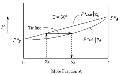
Consider a mixture of hexane (A) and heptane (B). Since both of these liquids are volatile, we expect that the solution too will have a vapour pressure. The vapour will be made up of a mixture of the two gases. The total pressure of this mixture, according to Dalton’s law is:

P^*_Soln  =  p_A  +  p_B   {sum of the partial pressures}

For Ideal solutions, we can determine the partial pressure component in a vapour in equilibrium with a solution as a function of the mole fraction of the liquid in the solution. This is Raoult’s law:

 p_A = x_AP*_A        and       p_B = x_BP*_B

Substituting into the first equation, we get,

P^*_Soln  =  x_AP*_A   +   x_BP*_B          or
P^*_Soln  =  x_AP*_A   +   (1-x_A)P*_B
=  P*_B  +  x_A(P*_A  – P*_B )

From this relationship, we see that the vapour pressure of a solution of A and B is a linear function of the mole fraction of A (or of B) where P*_B  is the intercept and P*_A  – P*_B is the slope.

The Vapour that collects over the solution will have a composition that is not necessarily the same as that of the liquid. The more volatile component evaporates easier and so will have a higher mole fraction in the vapour phase than it does in the liquid phase.
We can write

Mole Fraction of A in the vapour phase = y_A

Mole Fraction of B in the vapour phase = y_B

We can calculate these values from the solution concentrations using Daulton’s Law as follows.

The vapour composition curve can be plotted as shown in the figure below.  It is really two plots, one (the straight line) is the Vapour pressure of solution versus Liquid composition x_A and the other, (the curved line) is the same Vapour pressure of solution, but plotted as a function of Vapour composition y_A.  It could be thought of as pulling the Liquid line to the right (towards the more volatile liquid A).  Horizontal tie lines  join the two curves such that for any given Vapour pressure the liquid composition x_A and the the corresponding vapour composition y_A can be determined as indicated by the arrows in the figures.

Normally, we don’t carry out experiments as constant temperature as seemed to be indicated in the previous two figures and the corresponding discussion. To do so would involve complicated pressure measuring devices, sealed rigid containers and constant temperature devices.  We can much more easily do a measurement of temperature at fixed pressure (say one bar) as a function of mole fraction. We would thus get a plot of boiling point of solution as a function of mole fraction of the solution. To this, we can  add a plot of the vapour composition. This curve can be calculated using concepts much like those discussed above for the constant temperature case. The resulting curve (seen below) is shifted towards the higher vapour pressure component just as it was in the diagram above.

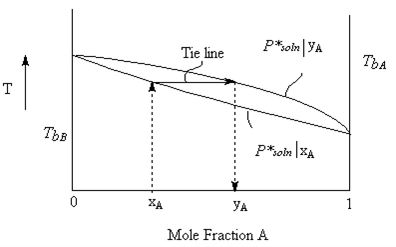
In this case, since we already know that the vapour pressure is not a linear function of Temperature (c.f. the Clausius-Clapeyron equation), we do not expect a straight line graph of boiling point as a function of composition. However, for an ideal solution the curvature of the line is only slight.

Let’s explore the tie line in further detail.  The graph of “T vs. mole fraction A” above has three regions in it.

1. Above the curves, is a single phase.  At any temperature and mole fraction condition, all components are in the vapour phase.
2. Below the curve, is a single phase.  At any temperature and mole fraction condition below the curves, all components are in the liquid phase.
3. Any Temperature/composition situation in between the two lines, there are two phases in equilibrium with each other.  One is a gas phase with component mole fractions y_i.  The other is the liquid phase with component mole fractions x_i.

For any experimental setup which has a point of temperature/composition that lies in between the two phases, we can calculate the relative amounts (total number of moles) of the two phases using the relative lengths of the tie line segments on either side of the point.  The diagram below is a blowup of the tie-line region of the previous figure; the blue line represents the liquid solution composition, the green line is the vapour composition.  The vertical axis is Temperature and the horizontal axis is Mole fraction of component A in a two-component mixture of A and B.  The vertical purple line represents the overall mole fraction of the system (both liquid and vapour phase).   The vertical position of the tie-line represents the temperature of the system.

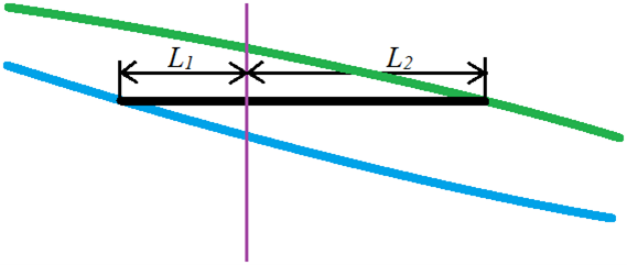
According to the lever rule (which was first developed for real levers but works here too), the length of the segment times the number of moles of the segment for one side equals the length times moles of the other side.

by rearranging this a bit, we can determine the ratio of moles of liquid to moles of vapour using the lengths and as follows:

This makes sense if we look at the graph.  If is shorter than (as illustrated), then the overall composition of the system is closer to that of the liquid that to that of the vapour phase.  That means most of the moles of material is in the liquid phase.

Example:  a closed system containing two volatile miscible liquids A and B is allowed to reach equilibrium.  The total number of moles of the system is 1.32 moles.  At equilibrium, 0.36 moles is found to be in the vapour phase. What is the ratio of lengths of the line segments and in a tie-line diagram as pictured above?

moles of liquid () = total moles () – moles of vapour ()

So, the ratio of the two line segment lengths will be 2.66.  Or, L₂ is 2.66 times longer than L₁.

9.4: Distillation

If we were to collect all the vapour above the liquid at the boiling point and then condense it we would have a liquid that was higher in the more volatile component than the starting material. If we then re-boil this liquid, we again increase the more volatile component in the resulting distillate.  With repetitive steps of boiling, condensing, boiling again, we can eventually completely separate the two components.  This would require, however an infinite number of steps.

9.4.1: Azeotropes

We have a more complicated situation in the case of two liquids, A and B, that mix completely but where the strengths of the intermolecular forces differ significantly. There are two possibilities:

1.  The average intermolecular forces in the solution is stronger than in the individual liquids
2.  The average intermolecular forces in the solution is weaker than in the individual liquids.

Since the intermolecular forces holding a liquid together determines the vapour pressure (and hence the boiling point of a liquid), we can predict that in the former case (1), the expected boiling point of the solution should be higher than that of either pure liquid while in the latter case (2), the solution will boil at a lower temperature than the boiling point of either of the two pure liquids.

Consider a solution of benzene and ethanol.  Benzene and ethanol are fully miscible but the intermolecular forces in the solution are less than that in the individual liquids. Since the forces holding the molecules are less, the energy (temperature) needed to break those forces are less.  Thus, we expect that there will be a minimum in the boiling point curve (see the figure below). at the minimum boiling point of the solution (mole fraction of ethanol = 0.46) we also find that the composition of the vapour is identical to that of the liquid. This is called an azeotropic mixture and the particular point on the boiling point curve is called the azeotrope.

A maximum boiling azeotrope happens when the intermolecular forces of the mixture are stronger than the individual liquids. This results in a mixture with a higher boiling point (lower vapour pressure) than the individual. In this case, vapour in equilibrium with the liquid have compositions away from the azeotropic mixture composition, towards pure liquid.

9.5: Solid Liquid Equilibrium

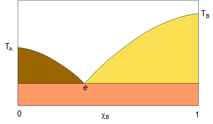
When we cool the solution system enough, we will reach the freezing point of the components and a whole new kind of phase diagram appears.  The solid/liquid solution phase diagram can be quite simple in some cases and quite complicated in others.   Let’s begin by looking at a simple two-component phase diagram with components that are fully miscible in both the liquid and solid phase. The diagram to the right shows a simple two-component A,B system solid-liquid phase diagram.  If we look at the diagram, we see several points indicated.  The vertical axis is temperature and the horizontal axis is the mole fraction (of B).  On the left side of the diagram, we see the freezing point of pure A, T_A , and on the right, the freezing point of pure B, T_B.  The white area is the liquid solution (aka the melt) with both A and B in liquid solution.  lines curving down from the melting points to a point labelled “e” are the melting point of the solution as a function of concentration.  Notice that in both cases, as you start from the pure component, A or B, and add the other component, the melting point goes down.  This is the effect we see in winter when we add salt to the ice to lower the freezing point. of the mixture so that the freezing point will lie below the ambient temperature and thus the ice will melt.  As the solution drops in freezing point, it comes to a common point, e, called the eutectic point.  This is the lowest freezing point for the system.  at any temperature below e, the system will be solid.  It will either be a mixture of crystals of solid A and solid B, or perhaps, if the temperature is dropped quickly enough, a solid solution of A and B.

In the white area of the diagram, there is only one phase, liquid solution.  In the coloured regions, there are two phases.  You can always identify the two phases by drawing a horizontal tie-line. the end points of the tie-line will tell you what each of the two phases are.  Take, the yellow triangular area.  If you draw a tie line somewhere in that region, you will have one end point on the curve that runs from T_B to e, and the other end on the vertical line at the pure B side of the plot.  So the two phases in the yellow area are the liquid solution and pure B solid.  In the brownish-green region, the two phases are liquid solution and pure A solid.  Finally, below the eutetic point, you will find two phases, solid A and solid B.  as I noted, this phase might be just a solid solution of A and B. The formation of pure crystals of A and B will only happen if the temperature is lowered through the eutetic point very slowly.

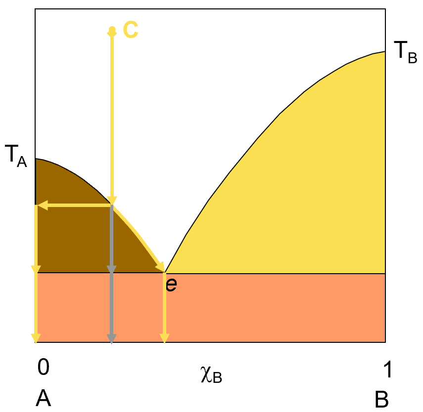
Let’s explore what happens if we have a solution of A and B and change the temperature so as to cause a phase change.  Obviously, the particular changes we observe will depend on the composition of the system.  Let’s start by exploring the result of dropping the temperature of a liquid solution of A and B as it freezes.  The diagram on the left shows such a transition.  IF we start with a liquid solution at point C, with the composition shown (about 75% A and 25% B) and lower the temperature of that solution, we will eventually reach the temperature at which we start to see solid forming.  This solid will at first be pure A (represented by the horizontal yellow arrow).  Because A is dropping out of solution, the solution concentration is getting richer in B and the freezing point keeps dropping as this happens, represented by the curved yellow arrow that follows the curve line down to the eutectic point.

If you keep cooling the solution to the eutetic point, you will have reached the point of maximum separation of A from the solution.  If you filter off the liquid at that point, you will be left with pure A solid and the liquid will be run off through the filter.  If you keep cooling the system past the point e, then the solution freezing point will hold steady until all the liquid has frozen out into a mixture of A and B solid and the average solid composition that forms from this further cooling will be that of the eutetic point composition.  The grey down arrow simply represents the overall system average composition but the actual materials you will find at any temperature will be represented by the yellow arrows.

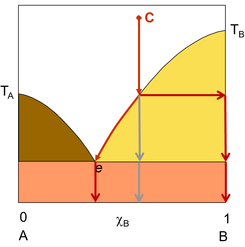
Let’s try that again.  This time, we’ll start with a liquid solution that is more concentrated in component B.  we start at point C with a solution that is about 60% B and 40% A.  As this solution cools (represented by the red arrows), it will eventually reach a point where pure B starts to solidify out of solution.  If you allow the system to continue to cool, more and more B will crystallize out until the solution reaches the composition e, where if you allow any further cooling, A will also start to crystallize out.  If you filter off the solid at any point at or above e, you will get pure B crystals and the remaining liquid solution will have some A and some B in it.  Just like we saw in the previous example, if you drop the temperature below the eutetic point, you will start to get both A and B in the solid phase and filtering will no longer be able to separate out a pure component.  your solid, below the eutetic point will be a mixtur of A and B.

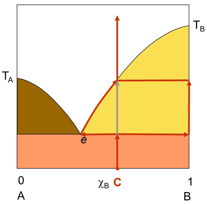
Let’s explore what happens if we start off with a solid solution of A and B. will start off with a solid solution of the same composition as we used in the previous example (about 60% B and 40% a).  The diagram on the left shows a red arrow starting at point C (solid mixture) and warming up.  When you reach the eutetic temperature, the temperature will stop rising as the solution starts to melt at the eutetic composition.  Eventually, the temperature will start to rise as all the A solid is all gone.  The only solid left will be B and any further melting results in a solution with a slowly shifting composition, richer in B as it melts.  Eventually, all of the B will be melted and you will have only a solution that has the same composition as the original solid solution had, unless you filter off the pure solid B somewhere between the point e and the point where all the B is melted.

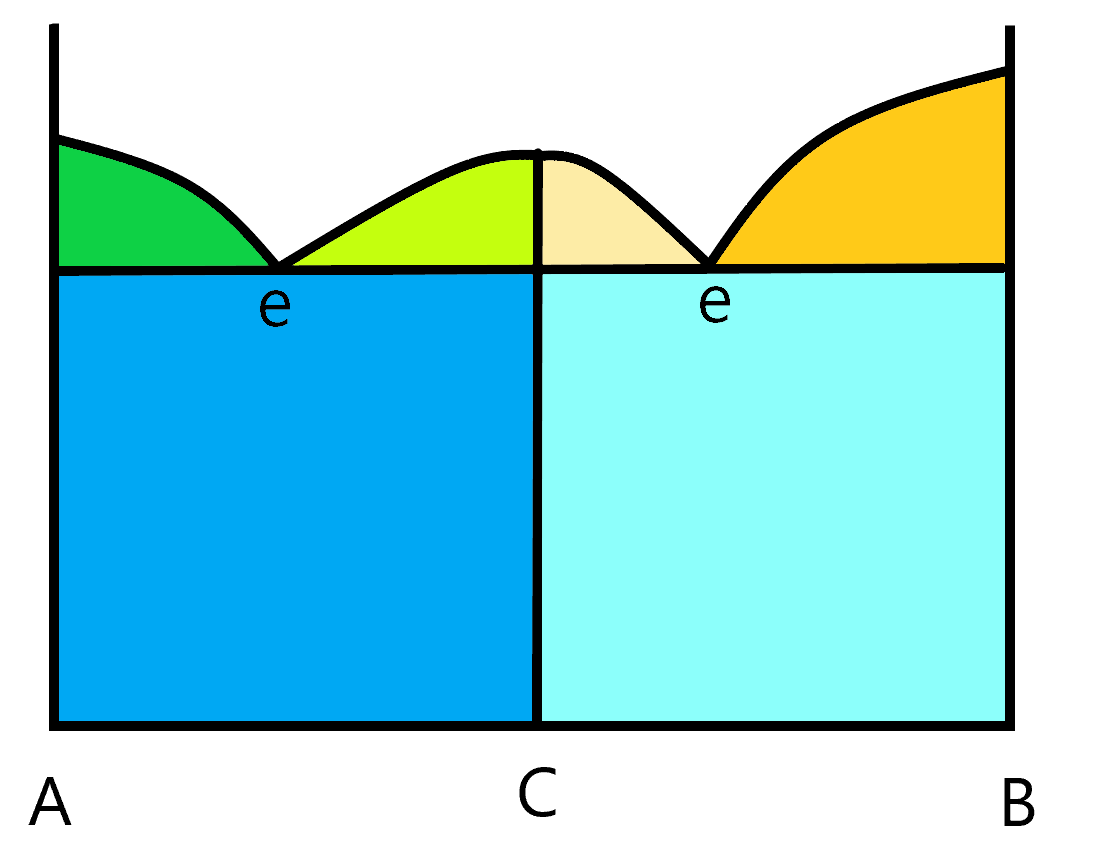
Not all phase diagrams are quite this simple.  There are a wide array of different kinds of phase diagrams, some more complex than the other.  This next diagram shows an AB system where, in the solid state, a new compound C is formed.  You can tell the composition of this compound by it’s location on the x axis.  In this case, it is exactly in the middle so it has equal amounts of A and B in the compound.  It’s emperical formula would be AB. Notice that because of the existence of this compound, the melting curve changes a bit.  If you start from solid pure C, and warm it up, you will reach a point where C melts into a solution of the same composition (but made of separated A and B).  This kind of compound is called a congruent melting compound. The melt and the solid are congruent with each other (meaning they have the same composition.  This results in two eutetic points.  In this simple diagram, the two eutetic points occur at the same temperature but that is not a requirement.  To understand the two components in any of the two component parts of the graph.  The green and orange triangular sections have two phases, one is the liquid solution and the other is one of the three compounds, A, B or C.  The two blue rectangular regions are two solid phase components.  The dark blue has A and C solid phases and the light blue has B and C solid phases as the two phases.  The white region above the melting curves have just one phase, the liquid solution.

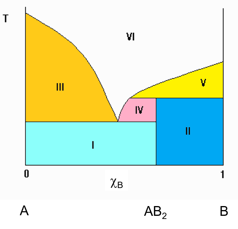
Sometimes, compounds that can exist in the solid phase will not melt.  They will decompose into other things before melting and you get was is called an incongruent melting compound.  This is a simple representation of an incongruent melting compound.  In the diagram to the left, you see a vertical line that is at the 2/3 mark of the x axis towards B.  this compound has a 2:1 ratio of B to A.  The emperical formula is AB₂.  Notice that the vertical line at this AB2 compound does not extend all the way to the melt as it did in the previous (congruent melting compound) diagram.  That indicates that AB2 does not melt into a solution of the same composition.  It breaks down before it melts, giving off a solution with a different composition and leaving behind, in this case, pure B solid.  This is an incongruent melting solid.  In this case, the different regions can still be identified by the horizontal tie line you can draw.

The regions in the diagram are numbered (roman Numerals).  As always, the white region (VI) is a single phase solution of A and B. The other regions (coloured) consist of the following components.

• I. Pure A solid and AB₂ solid.
• II. Pure B solid and AB₂ solid.
• III. Liquid solution and pure A solid.
• IV. Liquid solution and pure AB₂ solid.
• V. Liquid solution and pure B solid.

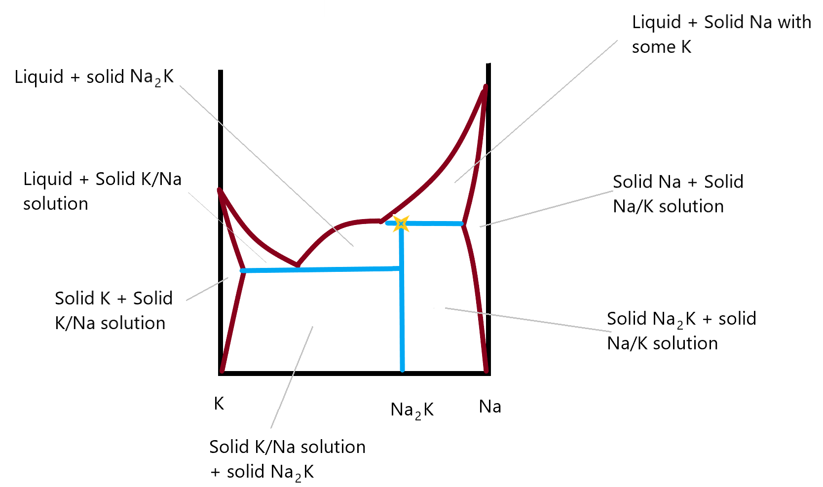
This final phase diagram shows a two component system made up of Na and K metals in different compositions. In this you can identify the incongruent melting compound and there are two new areas on either side, where you see that it’s possible to form a solid solution of Na in K (on the left side) or of K in Na (on the right side).  These metal amalgams are quite important in metallurgy as they are not just a mixture of the two solid phase components.  They are a genuine solid phase solution and the properties of the metal found in these regions differs from that of either of the two individual metal.  Most gold rings, for example are not pure gold but are an amalgam of gold and some other metal. This allows the resulting material to be corrosion free (like gold) but hard, (like the other metal in the amalgam, often silver.)  Back in the day when we all used thermometers with mercury in them, it was not uncommon to break one and have the resulting liquid mercury escape.  When cleaning up the mercury, you might accidentally touch your gold ring to the mercury and it would almost instantaneously turn greyish silver in colour.  That is the result of the gold/mercury amalgam that is formed.  Fortunately, you could reverse the process by heating the mixture, which would drive off the mercury. Unfortunately, the heated mercury can evaporate into the air where you might breath it in.   I once had a copper penny (we don’t have them any more) that had been dipped in mercury.  It had a silver colour to it like a nickel 5¢ piece.  I had it in my pocket for a long time to show people.  One day I noticed it was gone.  I wonder if I spent it as a penny or as a nickel?

If you cool a solution sufficiently, it will freeze. Allowing for the freezing to occur slowly enough and the solid which crystallizes out will be pure. The temperature at which the solution starts freezing depends on the composition of the solution. Take, for example, a mixture of acetic acid and water. Pure water freezes at 0℃ and pure acetic acid freezes at +16.6℃.  For the purposes of the following illustration, I wish to clarify the distinction between the word state and the word phase.

• A state is one of three states, solid, liquid or gas.  No distinction is given as to the material in that state.
• A phase represents a state where the composition of the material in that state is specified.

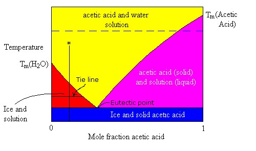
The phase diagram above shows four different colour coded regions.

• The yellow area is single-phase liquid solution.
• The blue area represents a single-state but two-phase region where solid ice and solid acetic acid crystals are mixed (might be solid solution or might not, assume not).
• The red area represents a two-state equilibrium between pure solid ice and a solution where the composition of the solution for any given temperature is represented by the position of the line which separates the red from the yellow areas.
• The violet area represents a two-state equilibrium between pure solid acetic acid and solution whose composition (for any given temperature) is represented by the position of the line separating the purple and yellow areas.

The intersection between the red-yellow border and the purple-yellow border represents the eutectic point. This represents the lowest melting point composition for this solution. For Acetic acid, water, that point is at a temperature of -26.7℃. Below this temperature, any mixture of ice and acetic acid is solid.

This diagram can be used to explain several kinds of phenomenon.

Suppose a liquid solution of with a mole fraction of acetic acid = 0.1 is cooled slowly, starting from room temperature. What phase transitions will occur as the cooling process progresses. Follow the vertical line (marked with an asterisk) at x = 0.1.

• The first phase change occurs at the temperature corresponding to the point where the vertical line crosses into the red zone. At this temperature, ice starts to crystallize out of the solution. This removes water from the solution, making it more concentrated in acetic acid. Hence, the freezing point lowers. This, process continues as the temperature is lowered such that the composition of the solution follows the red-yellow border down to the Eutectic point.
• Below the eutectic point both ice and solid acetic acid crystallize.

We use these properties in our every-day experiences, for instance, in the radiators of automobiles, we put a mixture of ethylene glycol and water. The correct proportions of these two compounds can give a solution that freezes at temperatures as low as -50℃. Even if it freezes, it will do so slowly, lowering the freezing point as it does and creating a slushy mixture rather than a single solid phase. Thus, even at extremely cold temperatures such as those found in northern Canada, the radiator ‘coolant’ mixture will flow through the engine and not plug it up.

Look at the diagram again. If we do an experiment at 10℃ (below the melting point of pure Acetic acid) in which we start with pure water and slowly add crystals of acetic acid, we can trace the progress along the blue dashed line.

At first, the acetic acid dissolves into the water. As the proportion of acetic acid increases, we reach the point where the dashed line crosses into the purple region. Beyond the purple-yellow border, we would see crystals of acetic acid sitting in the bottom of the beaker. The solution would be saturated (at equilibrium) and no matter how much more acetic acid solid we add to the beaker, there will be no further net increase in the amount that will dissolve. However, if we raise the temperature to room temp, we would see the rest of the acetic acid dissolve as we cross back into the yellow region on the phase diagram. Hence, we can use the diagram to determine the solubility (concentration at equilibrium) of acetic acid in water for any particular  temperature.

All phase diagrams of this sort have the same features. The pure liquids have characteristic melting points and the eutectic point represents the lowest melting point composition of the solution. There are always the same four regions and always, we can explain the freezing/dissolving processes using these diagrams.

In organic chemistry, we often use the properties of solutions to tell if we have properly separated out a desired compound. For example, in the synthesis experiments, which you do in the lab, you test the purity of the crystals you make by measuring their melting point. If your crystals melt at the correct temperature at a well-defined temperature, then your crystals are probably close to pure. If, on the other hand, they melt over a large temperature range or well below the correct melting point, you can be sure that your crystals are not very pure.

9.6: Solubility

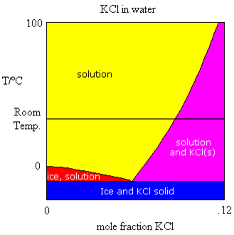
Sometimes, the components being mixed to form the solutions have melting points that are very different. Take for example, the mixing of water and a salt such as KCl. The salt melts at a very high temperature (770 ℃). The only part of the phase diagram which is of interest to us is the portion shown in the figure above. The same four regions are visible as we noticed in the water/acetic acid phase diagram. However, in this case, we are only looking at relatively low concentrations of KCl in water.

Let’s follow from (left to right) the horizontal line representing room temperature. As we add salt to our water, the salt dissolves at first. Salt will continue to dissolve as long as the concentration is in the yellow zone. Eventually, the salt no longer dissolves, it merely settles to the bottom of the beaker. The solution concentration that exists in equilibrium with the solid salt is represented by the intersection of the horizontal line with the purple-yellow border line. This is the solubility of the salt in mole fraction. We normally measure solubility in moles solute per litre of solution. We can easily convert the mole fraction determined here more common units, such as molarity. We can easily see that as the temperature of the solution is raised, the solubility goes up too.

We can also see that as the salt is added to the water, just like in the previous case, the melting point of the water is lowered. Hence, adding salt to ice on the sidewalks and roads lowers the melting point and (hopefully) the ice melts. In many parts of Canada, such as Saskatchewan, the temperature in winter is often well below the point where salt will do any good (~-20℃) and hence, it is rarely used there.

9.7: Henry’s Law

Common experiences tell us that gases dissolve in liquids too. For example, fish can live under water by separating dissolved oxygen from the water using their gills. If the water becomes stagnant and the dissolved oxygen content is reduced because of lack of aeration (mixing with air), many species of fish cannot live in it. Other species have developed special coping mechanisms for dealing with the low oxygen levels… But that’s another story.

We also see the effect of gas dissolved in liquid whenever we open a carbonated drink. The drink has carbon dioxide dissolved in it and while the can (or bottle) is closed, the pressure of the gas above the liquid is in equilibrium with the dissolved gas solution. This, of course is the vapour pressure of the CO₂ in the solution.   When the can is opened, the CO₂, whose vapour pressure is higher than normal ambient pressure, is released to the atmosphere and the liquid starts bubbling as the dissolved CO₂ starts evolving back into the gas phase. If we shake the can before opening it, the pressure of CO₂ above the liquid is raised noticeably, why^[1]?

We can see from this set of observations that the amount of dissolved gas in a liquid is dependent on two things. The first is the partial pressure of the gas above the liquid. The second is the rate of dissolution/evolution of the gas.

We are going to concern ourselves with the first option only and assume that enough time has passed to achieve equilibrium.

Henry’s Law expresses mathematically what we’ve seen experimentally.  It appears in form similar to Raoult’s Law

Where is the partial pressure of the gas  and is its mole fraction. is a constant that depends both on the solvent and the solute. It is called Henry’s Law constant.  Note, some books use or even for this constant.  Also, many other texts rewrite this equation in the form where the equation is inverted from the standard form and hence, so too will be the Henry’s law constants quoted in those books. Both those names have been replaced by IUPAC some time ago.

Table of Henry’s Law Constants for aqueous solutions.  is given in units of GPa at three temperatures.