Quantum Mechanics

Michael Mombourquette

6 Quantum Mechanics

Michael Mombourquette

6.1: Introduction

Newtonian physics deals with macroscopic (bigger than microscopic) objects and their interactions. It can deal with such things as inertia, gravity, collisions between large objects, etc. We are generally familiar with macroscopic physics concepts as described by Newton.

At the atomic level, Newtonian physics doesn’t work. Atoms are made of small (sub atomic) particles that do not obey Newtonian physics. Over the first half of this century, the theory now referred to as Quantum Mechanics, a.k.a., quantum chemistry, was developed. There are now several kinds of quantum mechanics theories. The earliest ones are now referred to as Classical Quantum Mechanics as opposed to more recent theories like Relativistic Quantum Mechanics. The most fundamental of these sub atomic particles, that we are interested in, is the electron. It’s thought to be indivisible. All of Quantum mechanics is based on this premise. In a recent issue of New Scientist, a report was published of an experiment which successfully split an electron into two smaller particles. If this report holds up under scrutiny, then Quantum Mechanics as we know it will need to be replaced with a new theory which allows for this to happen. This is all part of the scientific process, where we take our current models (understanding of reality) and metaphorically speaking, throw rocks at them trying to see if we can knock them down. The failure of a particular model is a good thing as it allows us to then develop new and better models and to know the conditions under which the old model may still be used.

These next few units will explore the various models that we need to understand as a basis to all of chemistry. We’ll start with small and very simple models and expand to more and more complex ones describing whole molecules and even macroscopic matter (crystals).

6.2: Nature of Light

Light has behaviors and properties that can be modelled in several ways, depending on the particular property we are observing or measuring. For example, light behaves as if it is made up of waves, when measured using appropriate experiments. The waves, in particular, are waves of electric field $\vec{E}$ and magnetic field $\vec{B}$ , as illustrated below. Some measurable properties of wave-like properties are the wavelength λ and frequency $\nu$ . The frequency and the wavelength are related to the speed of the light in a vacuum, c, according to the equation

$\lambda \times \nu = c$

The speed of light depends on the medium through which it is passing and it generally slows as it passes through a transparent medium, like clear glass, water or air. The slowing can be thought of on a microscopic level as resulting from the individual packets of light energy being absorbed and re-emitted repeatedly as it encounters the atoms of the material. The slight delay these absorptions and re-emissions cause ‘slows’ the progression of the light. The speed of the light in a medium v is related to the speed of light in a vacuum by the index of refraction of the material via

$n = \frac{c}{\nu}$

We don’t worry about the index of refraction or the variable speed of light in a medium very much in first-year chemistry but we should still be aware of the concepts.

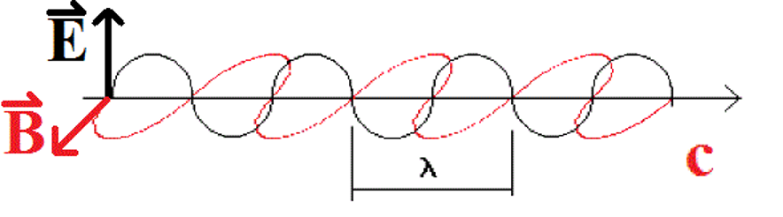Figure: One model of light shows waves of magnetic and electric fields alternating in a sine-wave pattern. Each field is oscilating perpendicular to each other. The two alternating fields together make up the light wave.

Light interacts with material when some property of the light matches a feature of the matter. For example, when the electric field oscillation of the light matches an electric field change in material then light can be absorbed as energy in to the matter. This happens in a microwave oven, where the polar water molecules in the food rotate at a frequency that matches the electromagnetic waves hitting it. The molecules absorb the energy and thus heat up.

light can also be absorbed when the magnetic oscillating field matches some property of matter. For example, in Magnetic Resonance Imaging, MRI, the magnetic nuclei of protons, which are oriented either with or against the field direction by the magnetic field of the big magnet, will switch orientations when just the right amount of energy of light hits it. This ‘resonance’ will absorb some of that light and hence the signal.

6.2.1: Electromagnetic Spectrum

We can see that the electromagnetic spectrum consists of a wide range of frequencies from radio-waves with wavelengths on the scale of mountain ranges and continents to gamma rays with wavelengths smaller than an atom. The visible spectrum makes up a very small part of this continuous range of wavelengths. Radio waves cover wavelengths as big as mountains and continents and as small as a person. Microwaves are smaller, generally in the centimeter lengths. Other types of light are shorter still.

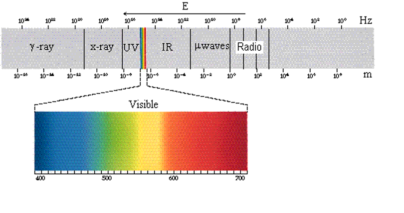Figure: The electromagnetic spectrum includes all types of electromagnetic radiation with wavelengths ranging from very long waves (10¹⁰ m) to very short waves (10^-16 m). We generally classify different types of light, depending on the wavelengths of the light. The boundaries separating the different types of light are not always well defined. types of waves are generally classified, from longest to shortest waves as: radio waves, microwaves (μwaves), infrared light (IR), visible light, ultraviolet light (UV), x rays and $\gamma$ rays.

6.3: Duality of Nature

There are two basic types of physical properties that can be used to categorize nature. These are:

Particles.
- Objects with mass and possibly charge.
- Can always measure position and momentum but not necessarily at the same time.
Waves.
- Periodic function (oscillatory motion)
- Cannot exist at a point, displaced over time and space.

Both matter and light have some properties (behaviors) that can be categorized as “wave-like” and other properties that can be called “particle like”. Electrons can be diffracted like light waves (electron diffraction patterns through metal foils) yet we think of them as particles. Light waves can behave like particles (photo-electron effect) yet we think of them commonly as waves.

6.3.1: Wave-Like Behavior

Where do we see wave-like behavior? Wave-like properties are observable in such experiments as

Interference patterns (addition/subtraction of waves)
diffraction (objects ~ same size as λ)
refraction (change in speed of light in different medium)

when we use lenses and mirrors and prisms to manipulate light, we are working with the wave-like properties of the light.

Even particles can exhibit wave-like properties. The electron microscope uses high energy electrons to illuminate material so it can be viewed on a very small scale. The wave-like properties of the electrons are being used here. The reason we need to use an electron beam rather than a light beam is that the size of the ‘waves’ of the electrons is very small compared to visible light and we can ‘see’ features in the matter that are the same size as the wavelength of the electrons.

Louis de Broglie proposed an equation that connects the momentum of the particle with the wavelength of the particle.

$\lambda = \frac{h}{p} = \frac{h}{mu}$

where $h$ is Planck’s constant, $p$ is the momentum of the particle, otherwise calculated as mass, m, times speed, $u$ . We use $u$ for speed in this case since the particle is microscopic. If we wanted to use this equation on a macroscopic particle (say, a baseball) we might use v for the speed but we would also calculate a wavelength that is substantially smaller than the size of the particle itself and hence would not be meaningful.

6.3.2: Particle-Like Behavior

The particle-like properties of light is known to exist. The solar system is clear of most interstellar dust and particles because light has momentum (even though it has no mass) and the momentum pushes on the matter in the solar system, sweeping it clear.

Here on earth, we can observe particle like behavior in several ways. Pigments and dyes are colored because the matter interacts only with light of particular energies. The fact that we can observe these particular energies means that the light itself has specific energies associated with it. This is not a wave-like behavior because if we could use waves to describe absorption of energy, then any wavelength of light would do for a given energy need, we would need only allow a long-enough string of light to be absorbed to ‘add up’ to the required energy. But, it doesn’t work that way. We see colours. That means the wavelength is connected to the energy of the light as an intrinsic property, and we cannot adjust the amount of energy by ‘cutting the string’ at different lengths.

To explain the ‘particle-like’ behavior, we consider light to be made up of wave packets, each of which can behave in some ways like a particle. The energy of such a packet of light, called a photon, is defined by the equation

$E = h\nu$

where $h$ = Planck’s constant and $\nu$ is the frequency of the light packet. The waves of light, are sine waves. Since sine waves are related to circular motion (yes, there is such a thing as circularly polarized light), we may wish to describe the frequency of light as a function of radians per second, rather than waves (or cycles) per second. Since, for every cycle of the circular motion, we undergo $2\pi$ radians of angle, we define this angular frequency ω as

$\omega = 2 \pi \times \nu$ .

Our energy equation, using angular frequency can be written as

$E=\frac{h\omega}{2\pi}$ .

We would like to make this a simpler equation to work with so we define a new physical constant called h-bar as follows

$\hbar = \frac{h}{2\pi}$ . ( $\hbar$ is also known as the Dirac Constant)

Thus we can now write our energy equation as

$E = \hbar \omega$ .

Photo-electron Effect

A particularly useful example of using the particle like behavior of light is the photo-electron effect. In this experiment, we observe that when light of sufficient energy strikes metal, electrons are ejected. By measuring the energy of the ejected electrons, we can perform some simple and interesting experiments.

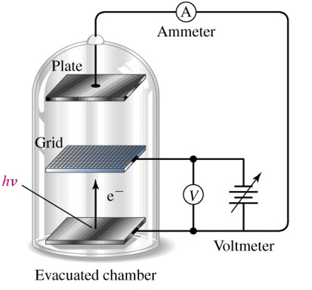Figure: The photo-electron effect involves a setup where we shine light on the surface of a metal. We can measure the kinetic energy of the electron by adjusting the voltage difference between the grid and the metal. If the voltage is too high, the electrons will be stopped and sent back to the metal. At a particular threshold stopping voltage, V_s, the electrons will be just stopped. Any lower voltage will not stop the electrons so we will be able to detect that as a current running through the apparatus. The exact voltage that stops the electrons depends on the frequency of light that we used.

The electron will generally require some amount of energy just to be extracted from the metal. This is called the work function of the metal (something akin to the ionization energy of a molecule) and is given the symbol $\varphi$ . If the particular photon that hits the metal and extracts the electron has more energy than the work function, then the excess energy goes into kinetic energy in the electron. The electron’s kinetic energy $(KE)$ is measured as the stopping voltage times the electron charge $(KE = e\times V_s).$ Thus, by using a series of different photon frequencies, we can determine the stopping voltage for each experiment and from that extrapolate to find the point where $(KE=0).$ This is called the threshold frequency $(\nu_0),$ where the energy of the photon exactly equals the work function of the metal $(h\nu_0 = \varphi).$ At higher energy experiments, we can equate the photon energy to the sum of the work function and the excess kinetic energy

$h\nu =KE + \varphi$

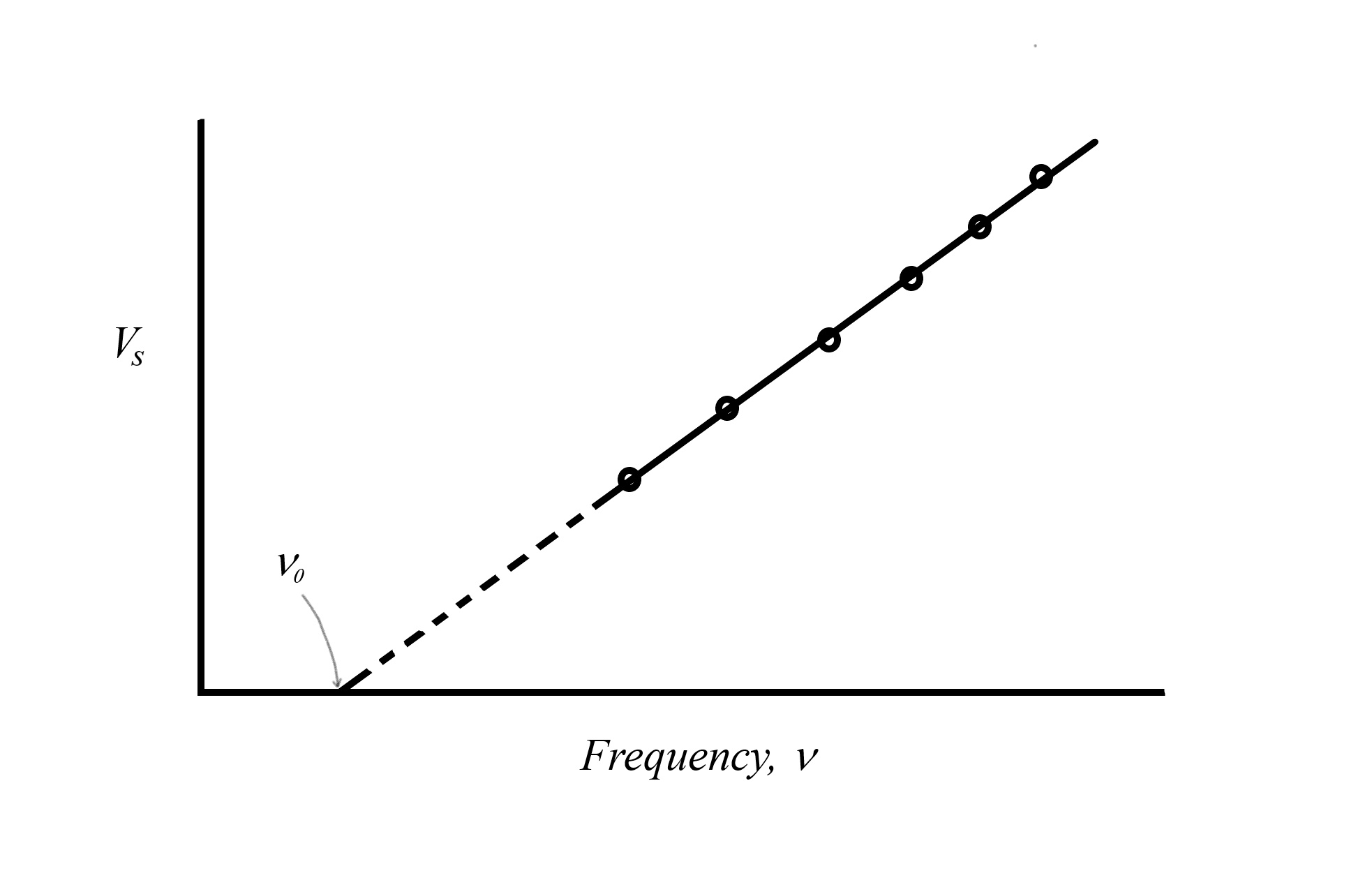Figure: Graph of the stopping voltage versus the frequency of light used in a photo-electron experiment using an apparatus like the one pictured above. The circled points represent data points from individual experiments where a particular frequency of light requires a particular stopping voltage. If we replotted this data with energy on the vertical axis, rather than stopping voltage ( $E = eV_s$ where $e$ is the electron charge) we would get a line with a slope exactly equal to Planck’s constant $h$ .

6.4: Quantization Effects in Nature

We normally experience the macroscopic world (larger than a microscope) where our observations are of measurables that are merely averages of the microscopic particles that make up the the matter. For example, we can easily measure the average kinetic energy of a gas (temperature), the momentum of a moving object, etc. Using light, we can probe the quantization inherent in atoms and molecules that we cannot otherwise detect with our own senses.

6.4.1: Hydrogen Atom

The ancient Greeks imagined the atom as the smallest indivisible particle of matter. They had no means of exploring that idea further than thought experiments. Early Scientific models of the atom included JJ Thompson’s model whereby, he knew, from experiment, there were both positive and negative particles in the atom. He imagined they were randomly dispersed in the relatively spherical atom. We call this the plum pudding model with the particles dispersed like plums in the pudding.

Rutherford tried to elucidate this idea further using an electron beam aimed at a very thin gold foil in an attempt to see the scattering from the atom’s positive and negative particles. He was amazed when he noticed that some of the electrons bounced back. He likened the discovery to “…firing a cannon at a piece of tissue paper and having the ball bounce back at you…”. His Model to explain this observation required that the all the positive charge be concentrated into a dense core we call the nucleus with the electrons circling around the nucleus, he imagined, like the planets circle the sun. This model didn’t stand up to several thought experiments however. For example, to constantly circle, the electron would need to be accelerated (attracted around the centre). But this very action would necessitate that some energy would be lost as radiation and hence, the electron would spiral down into the nucleus. Since electrons do not collapse into the nucleus, his model could not stand. Additionally, as we’ll see in the next paragraph on the Hydrogen atom, Quantization was observed in Hydrogen atoms and Rutherford’s model could not explain that as it allows that the electron could orbit at any distance from the nucleus.

See the source image — This is a typical drawing of the Rutherford model of the atom. electrons are shown orbiting the nucleus at random orientations and energies.

We begin our exploration of quantization with the hydrogen atom, the simplest of all atoms and the only one for which we have exact (analytical) equations that describe the energy states. When Atomic emission spectra (and absorption spectra) of Hydrogen atoms were studies, discrete frequencies of light (lines on the photographic paper) were found in the resulting spectrum. It was reasoned that those lines were connected to the atomic structure of the hydrogen atom itself. If there were discrete energies of light then there must be discrete energy levels in the atom itself. So, the atom is quantized in energy. But how to explain that?

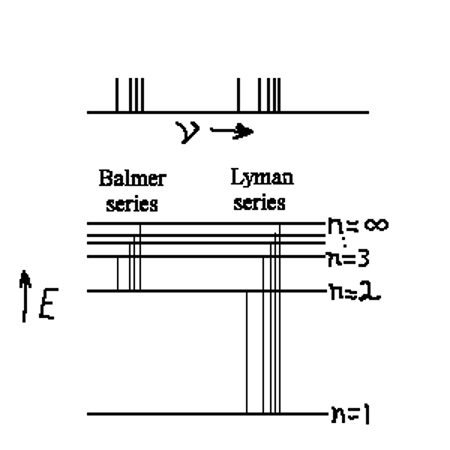
Emission spectrum H-atom

	$\leftarrow$ Hydrogen Spectrum
	$\leftarrow$ Energy levels with transitions shown lined up with the spectral lines.

The diagram above shows a spectrum from an emission spectrum as a series of lines. Each line represents a set of energy levels, each with it’s own value of n. This number n labels the energy level in the atom and is called the principle quantum number. In a hydrogen atom, that is all we need to accurately identify all the transitions in the emission spectrum. There are shown in the diagram two series of lines, the Balmer series and the Lyman series. The Balmer series lies mostly in the visible part of the electromagnetic spectrum and were observed first. This is the series of lines that all have n=2 as their lower energy level. As technology developed that allowed the study of the ultraviolet frequencies, the Lyman series was observed. The Lyman series all have n=1 as the lower energy. This larger drop, down to n=1 is why all these lines are in the UV region of the spectrum and into the infrared region is another series of lines called the Paschen Series (not shown in this diagram). This series all has n=3 as the lower level. In the far-infrared part of the EM spectrum one can find the Brackett series of lines, all of which have n=4 as their lower energy level.

6.4.2: Rydberg Equation

Rhydberg was able to quantify this pattern in the energies of the light using integer numbers n as a label for the energy levels in the atom. The Rhydberg equation is useful to determine the energy difference between two different energy levels in a hydrogen atom. When an electron jumps from one level (n₁) to a different one (n₂), there is an energy transfer involved. This energy could be thermal or it could be photon energy. In this case, I’ll use E to represent the energy of the photon of light emitted when this energy is given off as a photon.

$E = R_H\left|\frac{1}{n^2_1} - \frac{1}{n^2_2} \right|$

This equation gives the energy change when an electron moves from electronic energy level n₁ to n₂ or vice versa (note the absolute value signs), for an individual atom of hydrogen. One can easily determine the wavelength of the emitted (or absorbed) photon of light that is associated with this energy level change by dividing by Planck’s constant

The symbol $R_H$ represents the Rydberg constant and has a value of $\approx2.179\times 10^{-18}$ J. The magnitude of the change in energy of the hydrogen atom $\Delta E$ is the same as the energy of the photon emitted or absorbed in the process. The absolute value symbol means this equation does not distinguish between an absorption process $(n_1<n_2)$ and an emission process $(n_1> n_2)$ .

The Rydberg equation is a phenomenological equation. That means that it models the observed phenomenon, the discrete energy pattern observed in the H-atom spectrum (and other one-electron ions); but that there is no theory behind it. It simply works! We need to try to develop models that explain the observed behavior as described in the Rydberg equation. One such model is the Bohr model.

6.4.3: Bohr Model

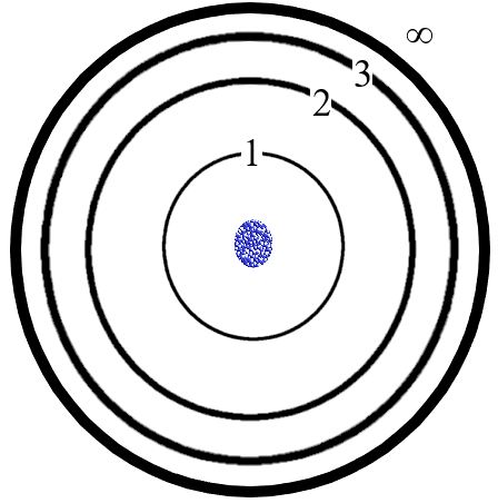
Figure: The Bohr Model produces a picture of an atom somewhat like the diagram above. The rings represent the orbits. Note that as n increases, the separation of the rings gets less and the n=infinity ring is not actually much further out than n=4 or 5. The upper rings (energy levels) are all so close together as to be unmeasurably close so that the lines in the spectrum at the upper end of any of the series (Lyman, Balmer…) is blurred out into a continuum of wavelengths. Bohr’s model is an improvement on Rutherford’s model in that now, electrons can only orbit at distinct distances (energies) but it still fails for multiple reasons, some of which also are failures in Rutherford’s model.

Bohr proposed a model, which explained the Rydberg equation.

It consisted of circular discrete orbits labelled $n = 1, 2, ... \infty$ .
$n$ is called the principal quantum number.
Each orbit represents one energy level.
The zero in energy corresponds to $n=\infty$ , i.e., when the electron is not associated with the nucleus, so all atomic energies are negative since the electron gives off energy when it drops into the grip of the atom.

Bohr was able to use classical mechanics to describe the energy levels. Using Columbic interactions between the electron and the nucleus and using the concept that the electron’s angular momentum is quantized and must be a multiple of $\hbar = \frac{h}{2\pi}$ (pronounced h-bar), he was able to calculate the Rydberg constant using fundamental constants.

$R_H = \frac{m_ee^4}{8\varepsilon_0^2 h^3 c\left(1 +\frac{m_e}{m_p}\right)}\times hc$

The “ $\times hc$ ” at the end of the equation is to convert the units from m^-1 to J. While Bohr’s model did a good job of working out a set of rules that accurately described the quantization of a hydrogen atom, it could not explain why the electrons did not simply spiral down to the center (nucleus) and continuously lose energy. It also fails to accurately calculate energies for anything other than a one-electron atom or ion. We’ll also see that it fails on a few more experiments as well.

Example: What the is energy and wavelength of a photon emitted when an e^– drops from the n=4 to n=2 energy level in a H atom?

$E = 2.179\times 10^{-18}J \left|\frac{1}{4^2}-\frac{1}{2^2}\right|=4.08_{56}\times 10^{-19}J$

$E_{photon}=4.08_{56}\times 10^{-19}J$

The wavelength can be calculated easily using the non-rounded value (keep the subscripted digits).

6.4.4: Heisenberg’s Uncertainty principle

One further failing in the Bohr model (and Rydberg equation) occurs in that the energies supposedly can be calculated analytically. The only limit of accuracy is in the equipment used to make measurements. The more accurate our instruments, the more accurate can we measure the energies of those transitions, according to the Rydberg equation.

Heisenberg, however, showed that there is an inherent uncertainty built into nature itself. The fact that we can have atomic spectroscopy means that light is acting in some ways as particles (a.k.a. photons). An individual photon of just the right energy interacts with an individual electron and we have an absorption (or emission). If light were just a wave, then we could simply hold the beam on the electron long enough for it to absorb enough energy and then it would jump to the required energy level. This is not what is observed experimentally, so light cannot be “just” a wave. But, we knew this from our discussion above of the duality of nature.

In order for light to be a packet of energy, rather than just a single wave, it must have, reasoned Heisenberg, a spread of waves with wavelengths all centered closely about the nominal wavelength of the beam. This would make for a series of overlapping waves that move in and out of phase with each other. When the waves are in phase, they positively reinforce each other to build up a packet of energy but when just a few wavelengths later, they are out of phase, the overall wave function is zero and hence, a boundary between the wave packets.

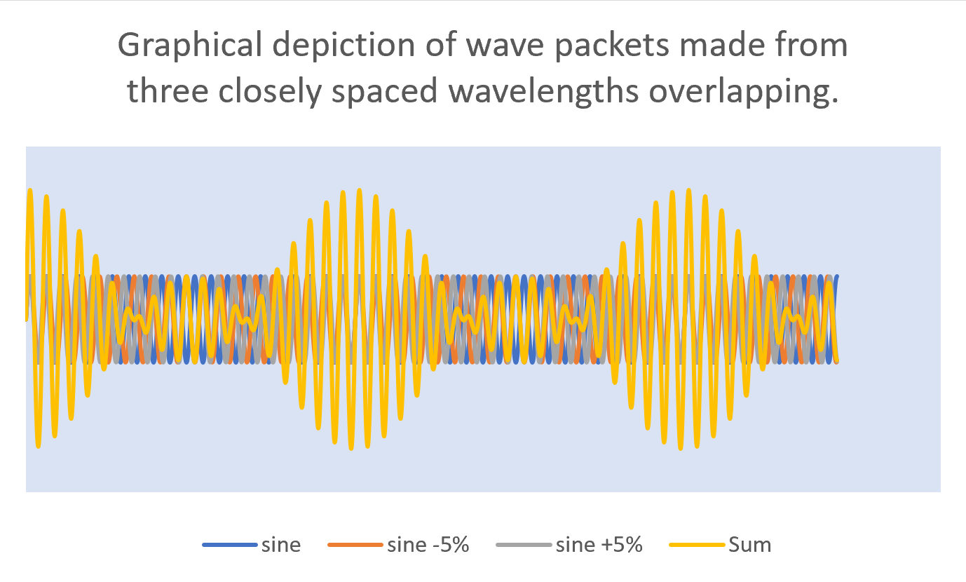In this image, we see four different waves. The first wave (in blue) is a simple sine wave (we will call this the principle wave). The orange wave is also a sine wave but one which has a wavelength that is 5% shorter than the principle one. The grey wave has a wavelength that is 5% longer than the principle wavelength. The yellow wave is the sum of the first three. It clearly shows a beat pattern that we can think of as a graphical representation of the wave packets. It’s one of these packets that contains the energy $E = h\nu$ where $\nu$ is the principle frequency.

A real wave packet in nature would be an overlap of many waves, all centered about the central principle wavelength, not just three waves, like I showed in the image above. The spread of wavelengths (spread of frequencies) means there is an uncertainty in the energy of the wave packet. The value of E that we calculate in the equation $E = h\nu$ , cannot be known exactly.

Heisenberg was able to determine that the value of the uncertainty can be related to the inherent uncertainty of the momentum and of the position of the particles. In one dimension (x), the uncertainty is

$\Delta p \times \Delta x \geq h/4\pi$

clearly, the more accurately we determine the position of a particle, the less we can know about its energy (momentum) and the more accurately we know the momentum (energy) of the particle, the less accurately we know the position. We cannot know both momentum and position accurately at the same time.

6.4.5: Multi-Electron Atoms

Rydberg and Bohr did a good job explaining the hydrogen atom and particularly, the quantization within the atom. Unfortunately, their model falls apart for anything else.

While other atoms also show line-type emission spectra, they are much more complex spectra that are not easily explained as was done for hydrogen. This is because there are more electrons and hence the calculations are more complex. To this day, there is no simple equation to describe the pattern of lines for any atom other than hydrogen.

Each atom displays a unique pattern of frequencies. This allows for a technique called Atomic Absorption (AA) to detect specific atoms. AA can detect atoms in stars and interstellar space.

6.5: Quantum Numbers

A more complete model needs more quantum numbers to fully define all the electrons in an atom:

: principal quantum number (q.n.) This quantum number labels the quantum level in the atom.
- $n$ = 1,2,3,…,∞
- $n-1$ is the number of nodes in any orbital in the $n$ ^th level.
: orbital (angular momentum) q.n. Essentially, this quantum number tells you what type of orbital you are working with.
- $\ell$ = 0,1,2,…, $n-1$
- indicates the number of nodes in the orbital that are angular. The rest must be radial nodes (spherical).
  - 0 angular nodes gives a spherical orbital, called s.
  - 1 angular node gives a dumbbell shaped orbital called p
  - 2 angular nodes gives a 4-lobed orbital called d
  - 3 angular nodes makes for an f orbital,
  - any nodes not counted here as angular will necessarily be radial (spherical).
: magnetic q.n.
- $-\ell$ ≤ $m_\ell$ ≤ $\ell$
- corresponds to the orientation of the orbital nodes.
  - Thus, for example, in p orbitals, there are three orientations of the orbital, often described in Cartesian space as $x,y,z$ . Since the quantum numbers are actually defined in complex space, there is no direct correlation of the values of $m_\ell$ with the real space $x,y,z$ directions. One would need to translate the complex functions into real space to find the connections. Don’t bother.
$m_s$ : electron spin (magnetic) q.n.
- $m_s$ = ±1/2
  - It turns out that if an electron is in an external magnetic field, it will orient it’s magnetic field in one of two orientations, either with the field or against it. These two orientations result in two slightly different energies for the electron (quantization). Thus, the two possible numbers for $m_s$ actually represent the direction of the electron’s magnetic field relative to some other field (often, some other electron’s field). So, if you have two electrons with the same value for their quantum number $m_s$ in an atom, they have their magnetic fields oriented the same direction to each other.

6.5.1: Spherical Harmonics and Quantum Numbers

To better understand the concept involved here, and to try to develop a picture of the concept discussed herein, let’s look at a series of macroscopic harmonic oscillators and see if we can find any trends.

1- Dimensional Harmonics

(The following is also called a “particle in a 1-d box”)

Consider the string on a guitar:

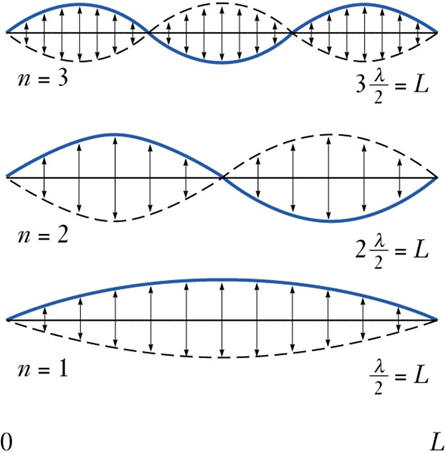
If the string vibrates with one continuous motion over it’s whole length, then it is vibrating in the lowest energy mode. We have a standing wave with length of $2L$ . If the string is prevented from vibrating in certain positions (nodes) the string will be forced to vibrate in a different mode. Each of these modes differs by the number of nodes in the wave function and in the frequency that results. (Listen). Note that to excite a particular mode of vibration, it is best to pluck the strung near the maximum in the vibrational wave function.

2-Dimensional Harmonics (drum skin)

Did you ever listen to a steel drum player? By tapping on different parts of the drum surface, they can make different notes. That’s because there are carefully placed dents in the surface of the drum that tends to damp out certain vibrations and which set up vibrational modes in the surface with maxima located in different places around the surface. By tapping in the location of a maximum of a particular vibrational mode the player can excite mostly that one mode and hence make that one note. By tapping a different place, a different vibrational mode is excited and hence a different note. Again the basic principal that the higher the number of nodes, the higher the vibration frequency is found to be true here in 2-d just like in 1-d sound.

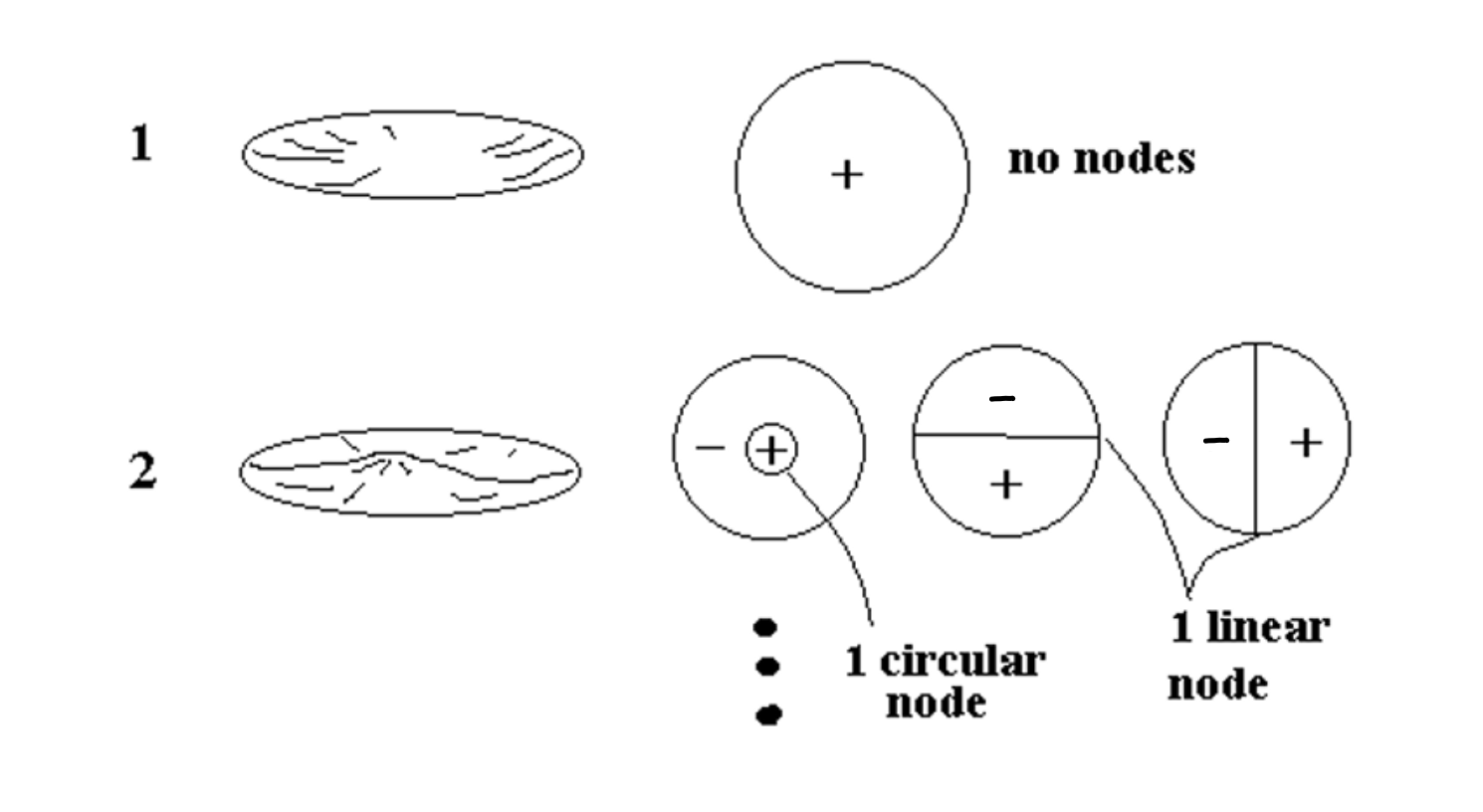
3-Dimensional Harmonics (spherical harmonics)

Harmonics in 3-d are not quite as easy to relate to musical instruments since most musical instruments are designed to vibrate in 1 or 2 dimensions, not three. Imagine a sound wave in a spherical container. Certain 3-d standing waves would tend to get established with high and low sound intensities at different regions and for different modes of vibration.

The basic types of nodes in the 3-d case are:

radial nodes, occurring at a specific radial distance from the center, resulting in a spherically symmetrical wave.
angular nodes, occurring at specific angles. These do not depend on the radial distance, only on the angle

It turns out that the properties of standing waves in a spherical system are very well described by a system of mathematics called spherical harmonics. This same mathematics works well to describe the electronic wave functions of hydrogen atoms. Erwin Schrödinger used these spherical harmonics in his equation to describe the atom as a nucleus with electrons existing around it as a series of these spherical wave functions. By doing this, he was able to retain quantization (and all the quantum numbers ) and also the wave function, which cannot be solved analytically, allow for some amount of uncertainty in the calculations, which now agrees with Heisenberg. Schrödinger’s equation looks like this:

${\cal H} \Psi = E \Psi$

This is a matrix equation where the $\Psi$ represents the full wave function of all the electrons in the atom and $E$ is the array of energies for all the states in the atom. The Hamiltonian ${\cal H}$ is an operator that incorporates the Coulomb’s law interactions between the nucleus and all the electrons and the electrons with each other, integrated over the 3d space of the atom (or molecule). For a further description of the wave functions, see Appendix 8.

Summary:

Notice that in all the previous cases, 1-d, 2-d and 3-d the following was true.

The lowest energy vibrational mode had no nodes (mode level 1)

The second level of vibration had one node (level 2) and in higher than 1-d, there were the possibility of more than one type of node.

The third level of vibration had 2 nodes, etc. Using the 3-d example, we can relate the nodes and their types to the quantum numbers discussed earlier. From now on, I’ll be discussing spherical harmonics as they relate to electron wave functions and I’ll be using the word ‘orbital’ to mean wave function. The type of orbital, obviously, is a function of the type (or lack) of nodes.

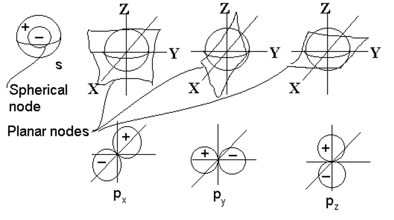
We have now seen that spherical harmonics describe the number of orbitals and also their shape. Let’s recap this information and relate it to the symbols commonly used to indicate the type of orbital.

The orbital quantum number $\ell$ describes the type of orbital. It gives the number of planar nodes in the orbital, and hence, defines its shape. While the number $m_\ell$ details its orientation. The shape of the orbital nodes can be determined from $\ell$ as follows:

$\ell = 0$ means no planar nodes (so, spherical orbitals)

$\ell = 1$ means 1 planar node (so, dumb-bell-shaped orbitals)
$\ell = 2$ means 2 planar nodes (4 lobed orbitals, except for the d_z^₂ orbital)
$\ell > 2$ means more complex shapes.

We can also use these numbers to count the total number of orbitals for any given value of the n.

$n$	$\ell$	$m_\ell$	type	# orbitals
1	0	0	1s	1

2	0	0	2s	1
	1	-1,0,+1	2p	3

3	0	0	3s	1
	1	-1,0,+1	3p	3
	2	-2,-1,0,+1,+2	3d	5

Electron Spin

Once we try to establish the actual electron count, we need yet one more quantum number. The electron spin is designated by the quantum number $m_s$ , which can have a value of +1/2 or -1/2

According to the Pauli Exclusion Principle, no two electrons can exist in an atom with the same set of these four quantum numbers. Another way of saying it; Every orbital can have at most two electrons in it and these two must have opposite spin.

Explains the electron count in the various shells of the atom:

$\begin{array}{|c|c|c|c|c|} \hline n=1 & \mathrm{one\; s\; orbital} & & & \mathrm{2\; electrons} \\ \hline n=2 & \mathrm{one\; s\; orbital} & \mathrm{three\; p\; orbitals} & & \mathrm{8\; electrons} \\ \hline n=3 & \mathrm{one\; s\; orbital} & \mathrm{three\; p\; orbitals} & \mathrm{five\; d\; orbitals} & \mathrm{18\; electrons} \\ \hline ... & & & & \\ \hline \end{array}$

Combining the functions which describe the electron with other energy-calculating functions (Hamiltonian) we can calculate the energy expected for any given function. The energy levels for an electron in a hydrogen atom can be calculated. These different calculated energy levels can be enumerated using quantum numbers $n$ and $\ell$ . If we add q.n. $m_\ell$ we now have a complete enumeration of the orbitals and q.n. $m_s$ finally enumerates the electrons.

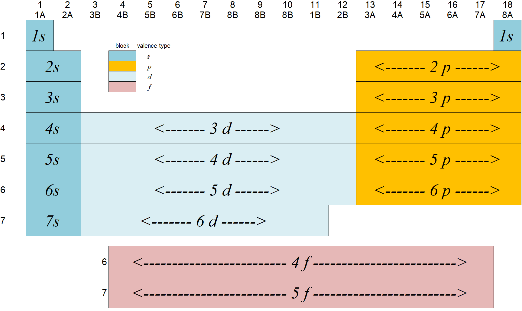
6.6: Periodic Table

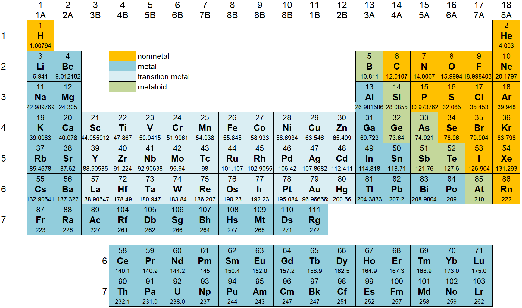
The periodic table shows the elements grouped according to the quantum numbers of their outermost valence electron.

The rows correspond to the principal quantum number n. The columns correspond (in groups) to l.

The groups (blocks) of elements in the periodic table are indicated as follows.

6.6.1: Electronic Configurations

To help understand the way the elements are organized in the periodic table, we need to see how electrons are located in the different atoms. We have two different basic concepts we need to work with in order to be able to work out the arrangement of the electrons: the Aufbau principle and the Pauli exclusion principle.

Aufbau Principle

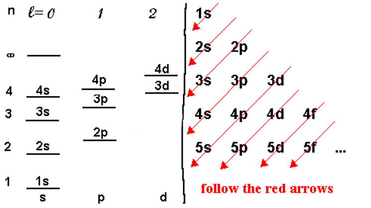
The Aufbau principle (or Aufbau process) simply states that the electrons in ground-state atoms will always occupy the lowest energy orbitals first and will only occupy higher energy levels when the lower ones are all filled. The energy levels for a multi-electron atom are depicted in the figure below left. In this graphical, we see that the energy of the levels generally goes up as n goes up but also there is an increasing trend as l goes up. As we get higher in n, the differences between the levels becomes smaller such that the higher l levels of one n level often are nearly the same or even higher than the lower l levels of the next higher n level. For example, the 3d energy levels are nearly the same or even slightly higher than the 4s energy levels for atoms that have 20 electrons or more. This is due to a process called shielding.

The Pauli exclusion principle tells us that there can be at most two electrons in a given orbital so we can now begin the process of filling up the electrons into the energy levels of the atom for whatever atom we are given.

We would fill up electrons by placing them (two per orbital) starting with the lowest energy levels and building up the electron configuration. A way to remember the sequence of orbitals without the need to draw the energy levels out in diagram form is to write the orbital identifiers (1s, 2s, etc.) as shown on the right of the diagram above and then draw diagonal arrows as shown in red. Starting at the top, the levels are filled in sequence as directed by the arrows. The number of electrons in any given set of orbitals is given as a superscript (1s¹ means one electron in the 1s orbital). Remember that some class of orbitals have more than one individual orbital. These are called degenerate (meaning same energy) orbitals. For example, there are three degenerate p orbitals so the set of p orbitals can have up to 6 electrons occupying them. Similarly, there are 5 degenerate d orbitals so there can be up to 10 d electrons and similarly, up to 14 f electrons.

Thus, a 15 electron atom (P), in its ground state, would be filled to give the following electron configuration.

1s² 2s² 2p⁶ 3s² 3p³.

Alternatively, we can follow the rows of the periodic table to determine the order of filling the orbitals. Unfortunately, we don’t always have such a reference with us and hence the memory technique is good to know too.

It is always important to recognize that these discussions apply to ground-state atoms only. For example, a hydrogen atom in its ground state will have an electronic configuration of 1s¹. However, if the Hydrogen is in an excited state (has more energy), that single electron will occupy a higher energy level. For example, 3d¹ is a valid electronic configuration for hydrogen. It’s just not a valid ground-state electronic configuration. Similarly, 1s²,2s²,2p⁴ is a valid electronic configuration for the ground-state oxygen atom while 1s²,2s²,2p³,3s¹ is one of an infinite number of valid excited-state configurations you might encounter for oxygen.

Note that levels 4s and 3d in the multi-electron atoms are very close to each other in energy. This also holds for 5s,4d and 6s,5d combinations. This leads to some exceptions to the rules normally used to assign the ground-state electronic configuration as we shall see below.

Examples: Using Aufbau process and Pauli exclusion principle, determine the ground-state electron configuration for the following:

H (1e^–) 1s¹

He (2e^–) 1s²

O (8e^–) 1s² 2s² 2p⁴

S (16e^–) 1s² 2s² 2p⁶ 3s² 3p⁴

Ti (22e^–) 1s² 2s² 2p⁶ 3s² 3p⁶ 4s² 3d²

Cr (24e^–) 1s² 2s² 2p⁶ 3s² 3p⁶ 4s² 3d⁴
If we strictly follow only Hund’s Rule and the Aufbau process, this is what we get. Experiment shows this to be incorrect. The correct electronic configuration for Cr is

1s² 2s² 2p⁶ 3s² 3p⁶ 4s¹ 3d⁵
or we can write it with the 3d and 4s reversed, as some people seem to prefer because after the Hund’s rule stabilization occurs, the 3d are actually lower than the 4s energy levels.
1s² 2s² 2p⁶ 3s² 3p⁶ 3d⁵ 4s¹

Cr is one of the exceptions. The 3d shell prefers to be half-filled (5 electrons) since this is a perfectly spherical configuration. There is significant relaxing of the energy levels in this configuration, such that the energy for the 3d electrons actually drops below the 4s energy. This type of situation arises whenever one can exactly half-fill or completely fill the d-shell.

Exactly filled or half-filled shells are spherically symmetrical and are more stable. In the case of the d-shell, since the s electrons of the next period are so close in energy, it is possible to promote an electron from the s shell to the d shell of the previous period, thus (half) filling the d shell. This filled (or half-filled) state is more stable and the d shell becomes lower in energy than the s shell of the next higher n level. Hence, the normal sequence of filling the orbitals is changed.

Shells	Half-filled	Filled
s	1	2
p	3	6
d	5	10

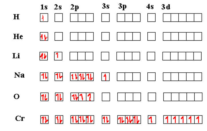
To illustrate these cases, we use box diagrams. A box diagram uses small boxes to represent the orbitals in an atom and arrows in the boxes to represent the electrons. The direction of the arrow (up or down) represents the spin of the electron (up spin or down spin; m_s = +1/2 or -1/2). At this stage, we need to introduce one more principle, Hund’s rule, to better understand the occupancy of the electrons in the orbitals.

Hunds Rule states that the lowest energy configuration for a multi-electron is one where the total electron spin is highest (for a given occupancy level of orbitals). Thus, if there are multiple orbitals with the same nominal energies (a set of p orbitals or a set of d orbitals, for example) then the electrons will occupy the orbitals one at a time with the electron spins parallel. After all the degenerate energy levels are half-filled, then, any additional electrons will occupy the same orbitals, but with the spins opposite from the first ones. We see Hund’s rule coming into play in the table of box diagrams below in atoms of O and Cr. Actually, the Cr seems to break the rules in that even the 4s orbital is half-filled.

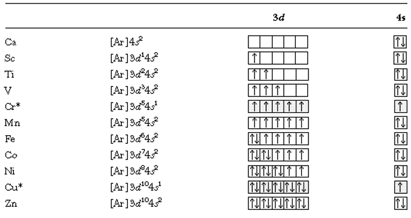
The Chromium atom has its 3d shell exactly half-filled in its most stable configuration. This can occur because the energy level 4s and 3d are nearly the same so the energy required to promote one 4s electron to the (slightly higher) 3d energy is more than compensated for by the lowering of the five 3d orbitals once Hund’s rule kicks in.

We would expect similar exceptions from the sequencing given above in other atoms in the Cr family. Also, exceptions occur in Cu and its family where the d¹⁰ configuration with one lone s electron is favoured over the alternative where one d orbital is half filled but the s has two electrons. Thus the electron configuration for Cu = [Ar]3d¹⁰4s¹ is lower than [Ar]3d⁹4s².

Electronic configurations for the metals in the fourth row of the periodic table (Ca-Zn). We see the results of applying Hund’s rule here as the total electron spin is kept as high as possible.* exceptions to the normal sequencing are indicated.

6.6.2: Trends in the Periodic Table

Now that we’ve seen the way that we can build up the electronic configuration of the atoms and how to organize the atoms into a periodic Table, according to their electronic configurations (quantum numbers) we can now look at some trends.

Atomic Radius

The first trend of import is in the atomic radius. The force of attraction between the outermost electron(s) and the nucleus affects the atomic radius. The force of attraction of two charges is given classically by Coulombs Law.

$F = \frac{kq_1q_2}{r^2}$

In the case of quantum mechanics, we cannot calculate a value for r exactly. And must rely on some mean value $<r>$ of the distance between the nucleus and the electron. Charges $q_1$ and $q_2$ represent the charge of the electron and the nucleus, respectively. For the purpose of discussing trends it is convenient to use the concept of core charge. The core charge represents the charge experienced by the outermost electrons of an atom, assuming the inner electrons shield the nucleus from their ‘view’. For example, in the atom Li there are two electrons in the ‘core’ shell (1s) and one in the ‘valence’ shell. The outer electron (2s¹) sees the nucleus (Z=3) only through the screen created by the two core electrons. Thus, it sees a core charge of Z – 2 = 1. More generally, the Core charge can be defined as

Core Charge = Z – # inner electrons.

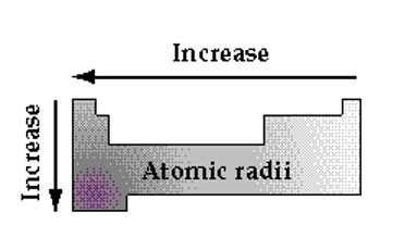
It turns out that, If we ignore the transition metals, we can simply take the column number to be the core charge. For example, Oxygen is in column # 6 and has a core charge of +6. Thus, along a given row, the orbitals are all approximately the same size, but the attraction of the electron for the nucleus (core) increases from left to right. Since the core charge increases from left to right along any one row, we expect the atoms on the right side to be smaller than those on the left because of the increased attraction to the core pulling the electrons closer. Similarly, as one descends a given column the core charge remain the same but the size of the orbitals increase.

Core Charge assumes that inner electrons shield the nuclear charge completely from the outer electrons. In reality, the orbitals in which these outer electrons exist actually penetrate the inner orbitals somewhat such that the effective shielding is not 100%. In addition, electrons in the same shell can partially shield each other somewhat. The amount of shielding and the final effective nuclear charge depends on differences in orbitals, and how they interact with each other. For example, s orbitals have more electron density near (or even on) the nucleus than a p orbital with the same principal quantum number and so shields the nucleus better (and is less effected by shielding from other orbitals) than the p.

Ionization Energy

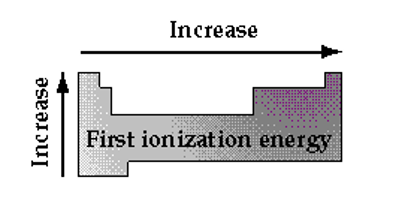
The First ionization energy of an atom is the energy required to remove one electron from the neutral atom as described by the equation below.

M —–> M⁺ + e^– ΔH = ionization energy

Arguments similar to the ones given for atomic size play a role here. This time, the larger the force of attraction, the larger will be the amount of energy required to pull the electron away. If we plot actual energies as a function of atomic number (or column in the periodic table, we can see this trend more explicitly.

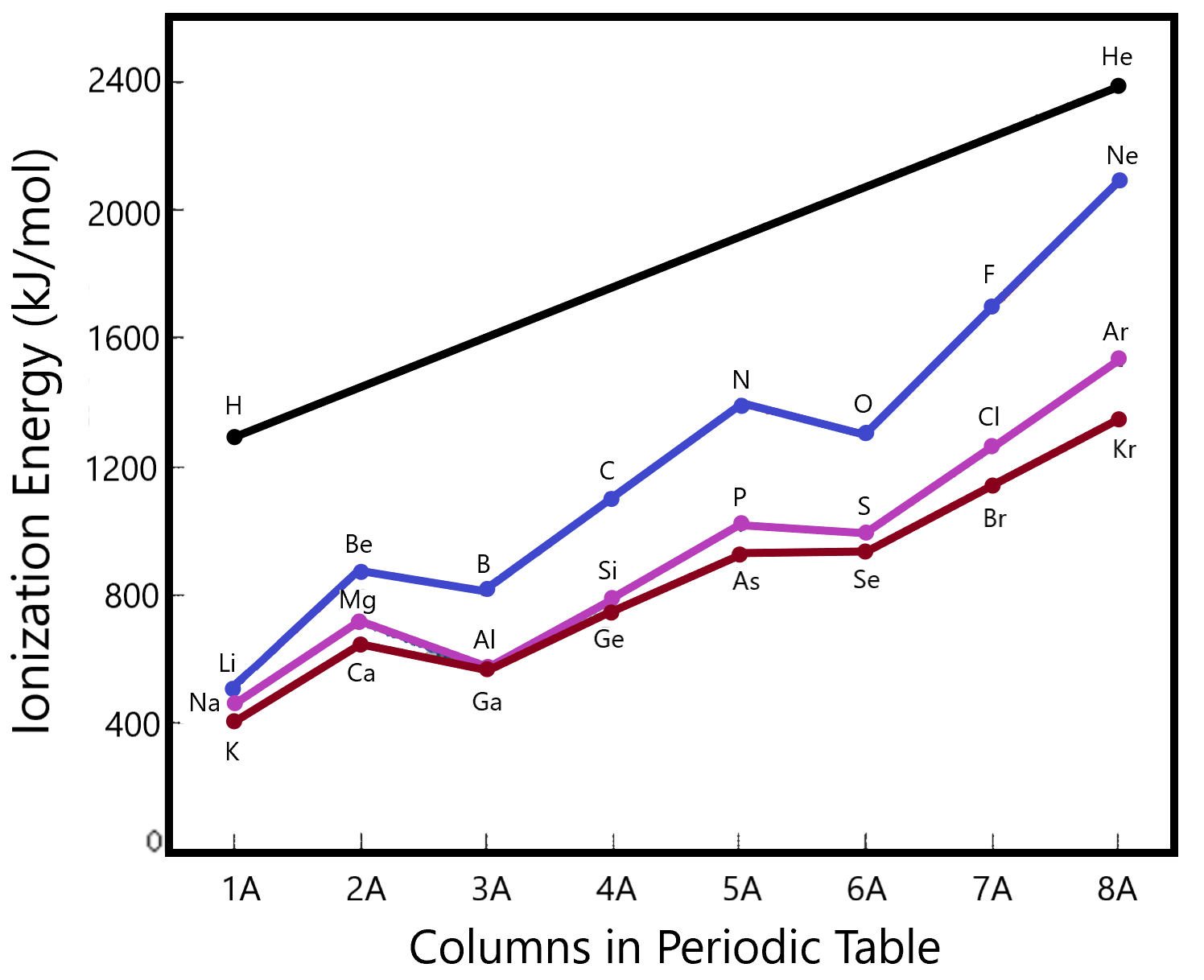
Note how the ionization energy increases as we go from left to right along the different rows of the table (colour coded). This follows the concept of Coulombic attraction. However, there are a few dips in the curve which bears considering. Be is higher than B (and Mg > Al, Ca > Ga as well). This makes sense since the former of each of these pairs represents the atom with a filled s orbital. The next orbital in the list is a p that is higher in energy (closer to the zero mark called completely removed). Thus the drop in ionization energies even though the force of attraction would be higher according to our first hand-waving discussion.

There is a similar drop in ionization energies as we move from column 5 to column 6. Here, we are transitioning from an exactly half-filled p-shell to one in which one extra electron exists. Since the half-filled shell is particularly stable, we expect a high ionization energy (for N, P, As…) whereas that for O, S, Se will be slightly lower (trend wise).

For second, third, etc., ionizations, the general trend within an atom is that each subsequent ionization is harder than the previous. This makes sense since each subsequent ionization represents the removal of a negatively charged electron from an increasingly positive ion (more attraction for the electron) and each subsequent electron is in a lower orbital on the given atom. For example, the second ionization energy is the energy required to remove the second electron from the atom, i.e., the energy to remove one electron from a +1 cation. Arguments similar to those for the first ionization energy hold when discussing the relative ionization energies of the various atoms.

Lets compare the relative ionizations of Na with Mg. Their first ionizations as plotted in the graph above show that Mg holds it’s outermost electron more tightly than Na since φ₁(Na) is lower than φ₁(Mg). However, when we look at the +1 ions resulting from these ionizations, we see that the Mg⁺¹ still has one electron in the 3^rd shell (It’s isoelectronic with Na) whereas the Na⁺¹ has its outer electron in shell 2 (It’s isoelectronic with Ne). It’s much harder to remove an electron from the second shell than from the third since the second is closer and more strongly held by the nucleus. So while there has been a large jump in difficulty in removing the second electron from the Na⁺¹, compared to removing the first electron from the neutral atom, there has only been a small jump in energy required to remove the second electron from the Mg⁺¹ compared to removing the first electron from the Neutral atom. Hence, the second ionization energy of Na is higher than the second ionization energy of Mg.

It’s dangerous to try to carry this type of argument too far into the levels of ionization of all atoms. There are too many factors involved to be able to perfectly explain all relative energy comparisons using any simple theory. More complete atomic orbital calculations would be required to precisely determine these energies.

Electron Affinity

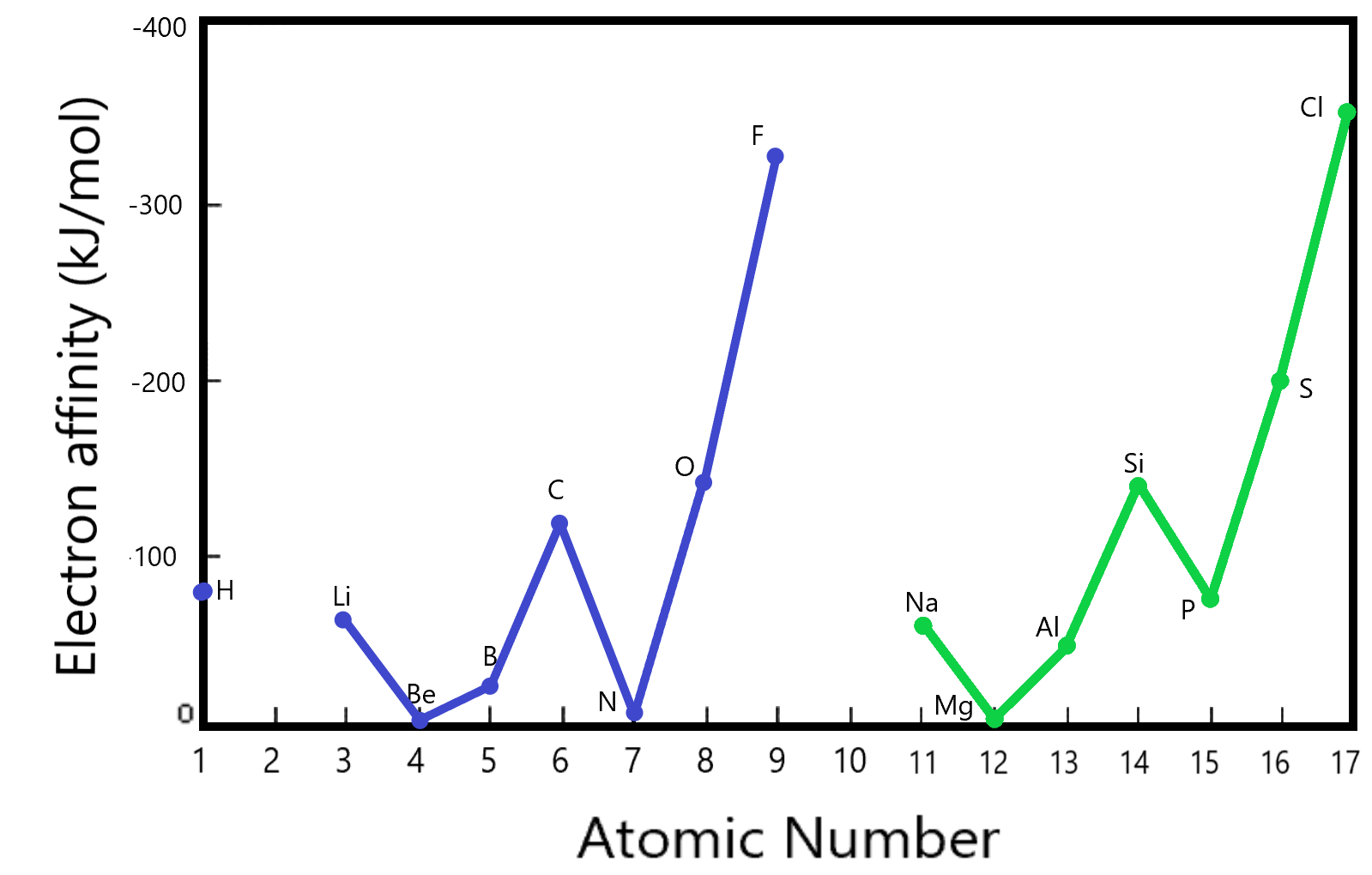
We can see a similar trend in the electron affinity comparisons. Electron affinity is the energy of attraction of the neutral atom for one extra electron. (How much energy does it take to add one electron to an already neutral atom as given by the formula below.

M + e^– $\longrightarrow$ M^– $\Delta H$ = electron affinity

(Note that $\Delta H$ can be thought of as negative of the ionization energy of the anion)

As we saw in the discussions on ionization energy, there is interplay between the relative size of the atom and the relative charge of the nucleus. The electron affinities listed here are for the first three rows in the periodic table (excluding the transition metals). We see that the highest affinities are displayed by the elements F and Cl (from the 7^th column). These belong to the Halogens. The Halogens as a family have the highest electron affinity of the elements. That also makes sense using Coulomb’s law wherein the Halogens experience the highest ‘core charge’.

One might ask: ‘Why do the Nobel gases not have a higher electron affinity than the Halogens?’. The answer lies in the fact that the Nobel gases have a completely filled outer shell and any extra electron added thereon would have to go onto the next higher shell which is of course higher in energy (not as attractive). These are not even included in the diagram above since they have virtually no tendency to form negative ions.

Reactivity

The reactivity of the elements in any one column (family) will tend to have similarities.

The elements in the first column are called the Alkali metals. The members of this family can all easily lose one electron to form a positive ion. These elements can often be found in salts such as LiCl, NaCl, KCl, … Their reactivity, although similar, will also differ since as they get lower in the periodic table, their outer electron is further and further from the nucleus and also, they are getting larger and larger. For example, Li(s) will react with water vigorously, Na(s) more so, and K(s) will burst into flames on dropping into water (even explode if too large a chunk is added).
The elements of the second column belong to the Alkali-Earth family. These tend to form +2 ions and salts of these metals combine with a different ratio than that of the alkali metals. Such compounds as BeF₂, MgCl₂, … belie the +2 charge on the metal. We’ll skip the transition metals for now. Follow the columns designated by A (see the periodic table diagram above)
The elements of the third column tend to form +3 ions except for the B case where a +3 ion of B would be very unstable. B does have a valence of 3, like all other column 3 atoms. It just makes covalent rather than ionic bonds, for example, BF_3. Here, the B-F bond is very polarAlCl₃ is an example of a Al⁺³ ion combining with three -1 chloride ions. Here, we see a significant break in the reactivity of the elements as we go from the first to the second row of the table. This tends to demark the boundary between metals (which form cations easily) and non-metals, which do not form cations easily.
In the fourth column, C is quite different from Si just as we saw in the third column. Yet there are still similarities. Both elements can form tetrahedral structures, as we’ll see later. Si tends to stand alone in that it does not act quite like C but it is also different from the lower elements in Column 4. The lower elements can all easily form cations (and are therefore metals). Si has semblance to the metals lower in the column and is there for classified as a semi-metal or metalloid.
In column 5, N and P both are non metals and can form -3 anions while As and Sb are classified as metalloids.
The 6th column (headed by O) is the Chalcogens family. Here, the first three elements are non-metals and can all form -2 anions. Te is the metalloid and Po is a metal. This is the only one of the elements in column 6 or greater to be classified as a metal.
In the 7th column (the Halogens), the elements tend to form -1 anions easily. They need only one electron to fill their outer shell and hence the strong tendency to -1 charge.
Finally, in the last column (the noble gases) the elements tend to be quite unreactive. Their outer shells are filled.

License

Icon for the Creative Commons Attribution-NonCommercial-ShareAlike 4.0 International License