Colligative Properties

Michael Mombourquette

11 Colligative Properties

Michael Mombourquette

11.1: Introduction

Colligative properties ⇨ Properties of solutions which depend on the number of solute particles but not on their nature.

Examples of colligative properties are:

Vapour Pressure lowering of a solution
Boiling Point elevation
Freezing Point depression
Osmotic Pressure

11.2: Vapour Pressure Lowering

The commonality in these properties is that the effects are entropy effects. Take, for example, the vapour pressure of a pure liquid versus one in which a solute has been dissolved. In the former case, the difference in entropy for the phase-change reaction is greater than that for the latter since the process of dissolving the solute into the liquid has slightly increased the entropy of the liquid (more random since the solute is spacing out the solvent molecules a bit).

Hence, the vapour pressure of the pure liquid is higher than that of the solution.

$P_{\mathrm{solvent}} = \chi_{\mathrm{solvent}} P^*_{\mathrm{solvent}}$

where P_solvent = vapour pressure of the solvent in solution,

$\chi_{\mathrm{solvent}} = \frac{\mathrm{moles\; of \;solvent}}{\mathrm{total \;number \;of \;moles}}= \mathrm{mole \;fraction \;of \;the \;solvent}$

and P*_solvent = vapour pressure of the pure solvent.
Recall that the total pressure of a solution is the sum of the partial pressures of the solvent and solute

$P_{\mathrm{solution}} = p_{\mathrm{solvent}} + p_{\mathrm{solute}} = \chi_{\mathrm{solvent}} P^*_{\mathrm{solvent}} + \chi_{\mathrm{solute}} P^*_{\mathrm{solute}}$

If the solute is non-volatile (no vapour pressure: P*_solute = 0) then the total vapour pressure of solution is

$p_\textrm{solution} = p_\textrm{solvent} = \chi_\textrm{solvent} P^*_\textrm{solvent}$

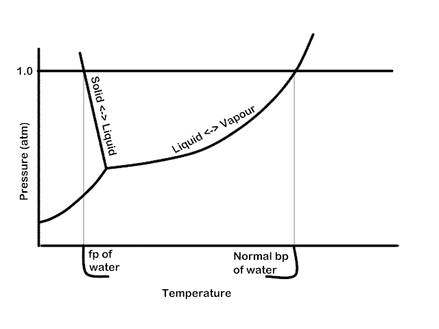
To see this in graphical form, see the phase diagram for pure water, below. Three lines are present indicating the phase transition (read equilibrium) between solid, liquid and gas. Where all three lines meet is the triple point where all three phases are in equilibrium. We see that at an external pressure of 1 atm. the normal melting point and normal boiling point are indicated. If the pressure is lowered, we note that the boiling point will be lowered and the melting point raised (very slightly; it’s exaggerated here).

Now look at the following diagram indicating the phase transitions for pure water and for water with some solute dissolved in it (not to scale).

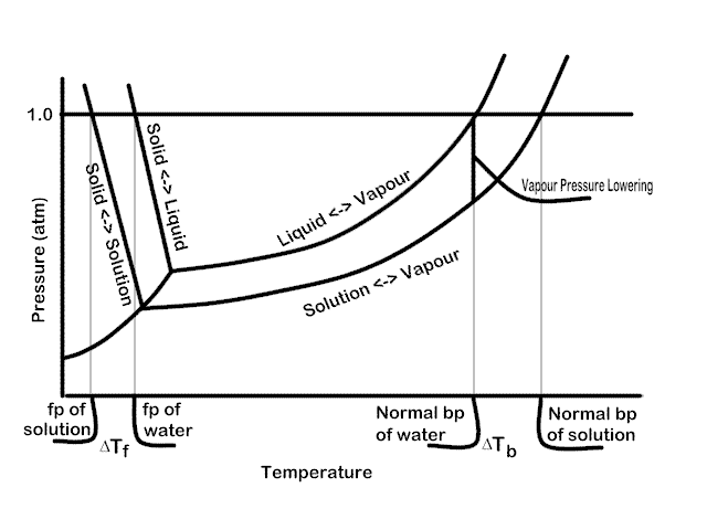
Here we see that the curves for equilibrium between the liquid and the other phases are lowered. Look, for example at the vertical line indicating the normal boiling point of water crosses the solution ? vapour at a lower pressure, i.e., the vapour pressure at that (and any other) temperature is lower for the solution. One could, in principle, calculate the concentration of solute which would be required to create a given VP lowering.

11.3: Boiling Point Elevation

We’ve already seen that in a solution, the vapour pressure of the solution is lowered. Thus, it is reasonable to conclude that one would have to raise the temperature of solution more to bring it to the boiling point. this point is well illustrated in the Phase diagram for water and solution figured above. There is a definite relationship between the concentration of solute and the increase in boiling point c.f. the pure liquid.

$\Delta T_b = k_bm$

m = molality of solute = # moles solute / 1000 g solvent

k_b = boiling point elevation constant for the liquid. We can use boiling point elevation measurements to determine the molar mass of an unknown solute.

Example:

A sample of 1.20 g of a non-volatile organic compound is dissolved in 60.0 g benzene. The BP of solution is 80.96℃. BP of pure benzene is 80.08℃. What is the molar mass of the solute.

ΔT = 80.96 – 80.08 = 0.88 ℃

$\Delta T \;=\;k_b m \;\;\Rightarrow\;\; m\;=\frac{\Delta T}{k_b}\;=\;\frac{0.88^oC}{2.35^oC\,kg\,mol^{-1}}\;=\;0.35 \,mol\, kg^{-1}$

but, we only have 60.0 g benzene, not 1000 g. so
# moles solute = molality × #kg solvent

$n\;=\;\frac{0.35\,mol\,solute}{1\,kg\,solvent}\times 0.060\,kg\,solvent\;=\;0.021\,mol\,solute$

$M\;=\;\frac{mass}{n}\;=\;\frac{1.20\,g}{0.021\,mol}\cong57\,g/mol$

NOTE: this is only an approximate molar mass, due to the inaccuracy of the measurement (small temperature effect, hard to measure accurately).

11.4: Freezing Point Depression

At the freezing point, solid and liquid are at equilibrium. The temperature where the equilibrium occurs at a pressure of 1.0 atm is called the normal freezing point. The same entropy effects which cause the boiling point to be elevated in a solution cause the freezing point to be depressed. See the figure above for a visual representation of this

Since at the freezing point, the solid and liquid have the same vapour pressure and since the vapour pressure is lower in the solution than in the pure liquid, it requires a lower temperature to achieve equilibrium. Actually, the solid’s vapour pressure too is affected by solute particles but to a much smaller extent than that of the liquid so we can ignore it for this hand-waving discussion.

The expression for the freezing point depression is: $\Delta T_f = k_fm$ where $k_f$ is the freezing point depression constant for the liquid and m is the molality of the solute.

Example

A solution of 2.95 g of sulfur in 100 g cyclohexane had a freezing point of 4.18℃, pure cyclohexane has a fp of 6.50℃. What is the molecular formula of sulfur?

$\Delta T_f = 6.5 - 4.18 = 2.32^{\circ}C$

$k_f = 20.2^{\circ}C\; kg/mol\mathrm{ (look up in tables)}$

$m\;=\;\frac{\Delta T_f}k_f}\;=\;\frac{2.32^o\mathrm{C}}20.2^o\mathrm{C\,kg\,mol}^{-1}}\;= \;0.115\mathrm{\,mol\,kg}^{-1}$

$\frac{0.115\mathrm{\,mol\,sulfur}}{1000\mathrm{\,g\,solvent}}\times100\mathrm{\,g\,solvent}\;=\;\mathrm{0.0115\,mol\,sulfur }$

$\frac{2.95\,\mathrm{g\,sulfur}}{0.0115\,\mathrm{mol\,sulfur}}\;=\;257\, \mathrm{g\,mol^{-1}}$

This is only the approximate molar mass of the since this technique is not very accurate (only 2 or three sig figs in this experiment).

Atomic molar mass of is 32.06 g/mol. It takes 8 atoms of to add up to about 257 g/mol. Thus, the molecular formula for is S₈ and the true molar mass is
8 × 32.06 = 256.48 g/mol

Example

How much glycol (1,2-ethanediol), C₂H₆O₂ must be added to 1.00 L of water so the solution does not freeze above -20℃?

$k_f (H_2O) = 1.86^{\circ}C\mathrm{ kg/mol}$

$\Delta T_f = k_fm$

$m\;=\;\frac{\Delta T_f}{k_f}\;=\;\frac{20.0^o\mathrm{C}}{1.86^o\mathrm{C\,kg\,mol}^{-1}}\;=\;10.8\, \mathrm{molal}$

since 1.0 L has a mass of 1.0 kg we need 10.8 mol of ethylene glycol

10.8 mol × 62.1 g/mol = 670 g ethylene glycol.

11.5: Osmosis, Osmotic Pressure

Osmosis is a process whereby liquids pass through semi-permeable membranes, spontaneously. This process is driven by changes in entropy. Consider two containers of liquid, connected by a semi-permeable membrane. The semi-permeable membrane can be simply a device which holes small enough to allow the solvent to pass through but not the solute. In one container is a pure solvent and in the other is the same solvent but with some solute dissolved in it. In this case, there will be solvent passing through in both directions randomly. The rate of the two processes depends on the relative entropy of the two sides and on the relative pressure applied to the solutions.

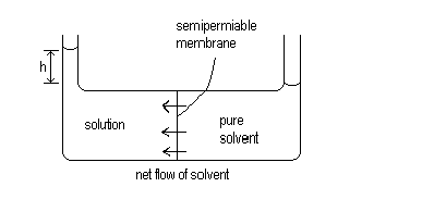
Since the solution will have a higher entropy than the solute, it is reasonable to expect that the spontaneous process is the one where the solvent passes through the membrane from the pure solvent side to the solution side where the entropy is higher. This will occur until the difference in the height of the two columns of liquid (h) is large enough that the pressure caused by this column of liquid exactly stops the net flow of solvent. This pressure is equal to the osmotic pressure.

Osmotic pressure is given the symbol $\Pi$ (Greek equivalent of P) and the equation relating the osmotic pressure to the amount of solute is:

$\Pi V = nRT$

Note that $n/V$ is concentration in mol/liter so we can also write

$\Pi = C_{M,solute} RT$

$\Pi$ can be measured at room temperature and is therefore, more useful for measuring solutes which might decompose at higher (boiling point elevation) temperature measurements. It is also extremely sensitive to small amounts of solute and is therefore useful for measuring very large molar mass values.

Example

An aqueous solution containing 1.10 g of a protein in 100 mL of solution has an osmotic pressure of
3.93 × 10^-3 atm at 25℃. What is the molar mass of the protein?

$n\;=\;\frac{\Pi V}{RT}\;=\;\frac{3.93\times 10^{-3}\,\mathrm{atm}\times0.100\,L}{0.08206\,\mathrm{L\,atm\,mol^{-1}\,K^{-1}\times 298\,\mathrm{K}}}\;=\;1.63\times 10^{-5}\,\mathrm{mol}$

Note that in this case, we used a different value for the ideal gas constant
$R = 0.08203$ L-atm mol^-1K^-1.
This is simply a convenience because the units cancel out to give the desired answer (work the details if you don’t believe). The alternate way is to convert to SI units.

$n\;=\;\frac{3.93\times 10^{-3}\,\mathrm{atm}\left( \frac{101.325\,\mathrm{kPa}}{1\,\mathrm{atm}}\right)\times0.100\,\mathrm{dm^3}}{8.3145\,\mathrm{J\,mol^{-1}\,K^{-1}\times 298\,\mathrm{K}}}\;=\;1.63\times 10^{-5}\,\mathrm{mol}$

now that we have the number of moles, the calculation of molar mass M is straight forward.

$M\;\cong\;\frac{1.10\, \mathrm{g}}{1.63\times 10^{-5} \,\mathrm{mol}}\;=\;67.5\,\mathrm{kg/mol}$

Note the very high molar mass of the protein.

11.6: Electrolyte Solutions

IF we dissolve NaCl in H₂O we get two ‘particles’ in solution for every one unit of NaCl. Since the Colligative properties depend only on the amount of solute, not on its nature, the concentration of the ‘stuff’ in solution is actually twice that of the nominal concentration of the salt. This must be accounted for in the case of electrolytes dissolving in water. We can use this idea to determine the amount of dissociation of weak electrolytes, we can determine the number of particles a given electrolyte breaks up into. If we assign the symbol i to be the number of ions an electrolyte breaks up into we can rewrite the colligative properties as follows:

$\Delta T_b = i k_bm$