Appendix 1: Propagation of Errors in Calculations.

Michael Mombourquette

Appendix 1: Propagation of Errors in Calculations.

Experimental Uncertainties

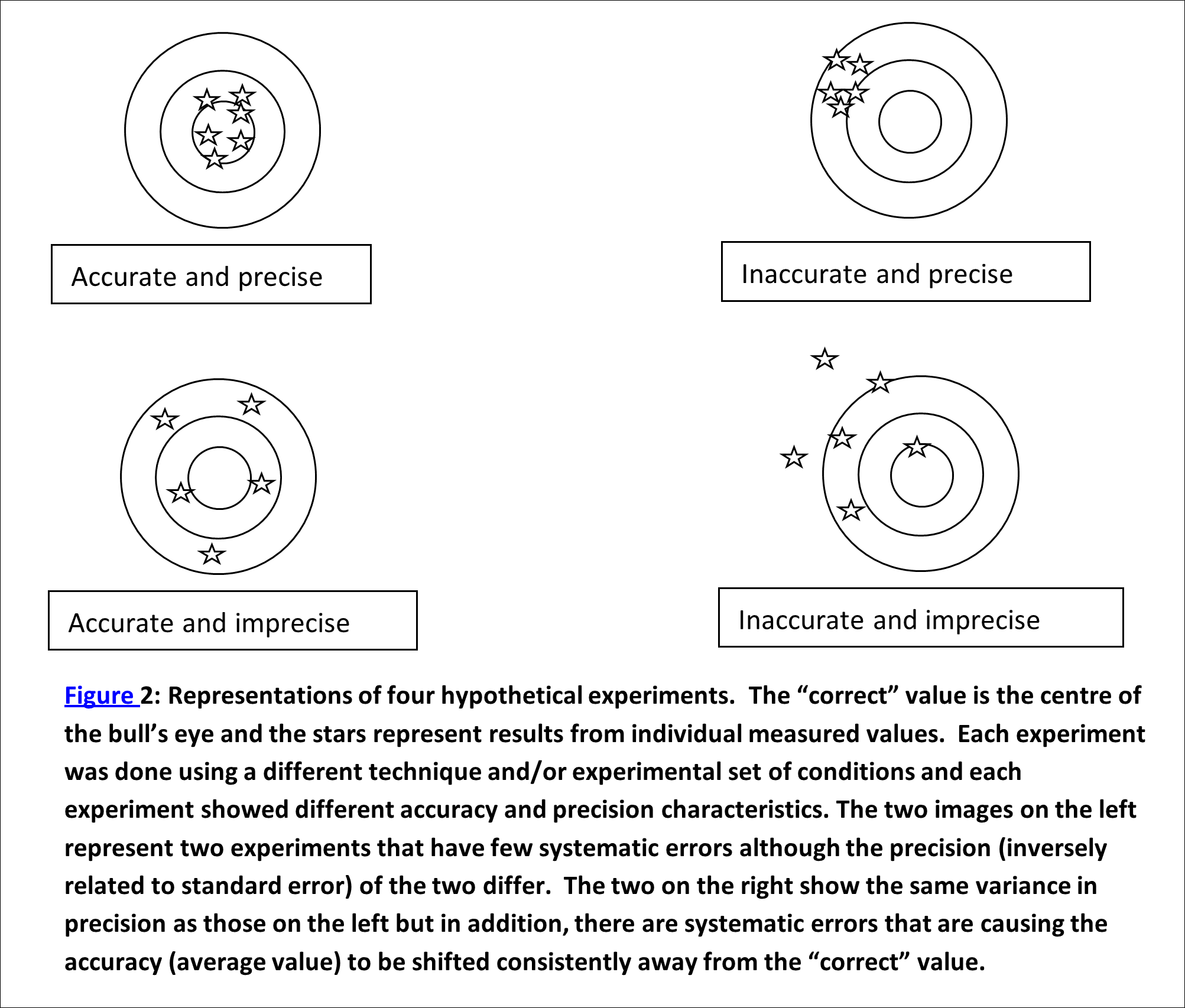
Every measurable (mass, length, time, etc.) has a “correct” value, even though we may never be able to determine it exactly, due to errors and uncertainties in our measurement (See Figure 2). We mostly settle for quoting the most reliable measurement we can make along with the uncertainty in that measurement.

Your goal is to make your measurements as accurately as you need for the purpose and quote the measured value and the uncertainty in that value. The uncertainty (or uncertainty limit) is usually dictated by the limits that your experimental equipment and techniques impose. All measured values should include a measure of the uncertainty inherent in the value. For example, a 50 mL burette has a standard uncertainty of 0.05 mL at 25℃, i.e., it can measure volumes to within ±0.05 mL. So, any volume measurement made using a burette should be written as (say) 1.30±0.05 mL or more efficiently as 1.30(5) mL^[1]. Here we see that the zero after the 3 is important and that the range of possible “correct” values is actually 1.25–1.35 according to our experiment. Typically, this uncertainty measurement defines the maximum uncertainty that we expect from our equipment or experimental setup.

Methods for determining estimates of experimental uncertainties:

Sig. Fig. method: Keep track of significant figures (on page 17). This gives us the crudest indication of uncertainty possible. Usually, the last digit in the reported number is assumed to be the one that is uncertain. For example, the number 2.54 might be 2.51 or 2.59. This is the simplest way to indicate the accuracy of a calculated or measured number. However, this method gives you only a “ball park” estimate of the uncertainties and is therefore the poorest way to keep track.
Propagation of uncertainties method: Record the individual uncertainty of each measured datum and then propagate the uncertainties (on page 18). This method is useful in cases where you can only do a single (or very few) experiment(s) with multiple measured numbers used in each experiment. This method always gives you the maximum uncertainty of a given calculated number. The actual experimental uncertainty may be less than what you calculate.
Statistical method: If your experiment allows or requires you to measure a large number of samples, you can do better than methods 1 or 2 and by using statistics to determine a mean and standard error (on page 20) of the results calculated from your measurements or standard errors on the slope and intercept if you are doing a graph. This last method is actually the best way to determine the actual uncertainty in your experimental results. It also works where you have no other way to identify the magnitude of the errors from the individual measurements.

Expectations for your written work

As a scientist (or science student), you will be expected to indicate the level of uncertainty in all measured numbers and any numbers calculated using those measured numbers in any formal writing/reports you produce over your career. You will be expected to keep track of Sig figs at all times according to Method 1 below, and you will be expected to use Method 2 or 3 for any quantitative experiment. Experiments or parts of experiments that are wholly qualitative need not involve uncertainty calculations.

Method 2 will have to be used in any experiment or report where you will only be working with a single set of measurements (or very few measurements) and from that, calculating a result. You will need to collect the individual errors from all measured values and propagate them to get an estimate uncertainty limit for the final result.

How do you determine uncertainty limits for individual measurements?

Documented uncertainty limits. Some devices list the uncertainty in the measurements taken using them. See the last page of the manual for a list of uncertainties on devices you will be using in this laboratory room (on page 159).
Analogue Scales: When reading from an analogue scale, such as volume markings on a burette or length markings on a ruler, you can typically measure to within ±20% of the smallest marking on the device (unless otherwise specified). Thus, if your ruler has millimeters (mm) as the smallest unit marked then you can measure to within ±.2 mm by estimating the final decimal place between the two marked mm units on the ruler (See burette example on page 29).
Digital scales: You can watch the small fluctuations in the reading and visually do the uncertainty calculation yourself. Let’s say, you see a meter reading of 0.163 but the last digit seems to jump up and down a bit between 0 and 6. You can infer from this that the last digit is in error by about ±3. The reading and error limit must be reported as 0.163±.003 or simply as 0.163(3). We often refer to this method as determining the uncertainty visually.

Method 3 can be used if you are collecting data sets from multiple trials to get an average or to create a straight-line graph. Then, you can use statistical methods to determine the uncertainty limits (a.k.a., standard error) and you do not need to collect individual uncertainties and propagate them.

Interesting point. The sig figs of a number implies that the last digit in the sig figs is the uncertain one. If your propagation of errors or statistical results gives an uncertainty that implies a different number of sig figs from what you got using just the sig fig method above, then the error calculations always override the sig fig method of determining the uncertainty.

For example, if my calculated answer is 123.456 but the sig fig count I get is 4, I would report the final answer as 123.4. If I do one of the two error calculations in method 2 or method 3 and get an uncertainty of 0.02 then the final answer would be 123.45+0.02 or written more succinctly as 123.45(2). So, 5 sig figs, despite my rudimentary determination of only 4 sig figs. The uncertainty calculations rule.

Systematic versus Random errors

The two types of errors that commonly occur in experiments are systematic and random errors (See Figure 2).

Systematic errors typically affect only the accuracy of the measurement and are due to defects in equipment or in the design of the equipment and the method itself; for instance a balance may be incorrectly calibrated, so that if the same balance is used for every measurement, every result is affected in the same way. Sometimes systematic errors can be avoided by using a range of different methods for measuring certain quantities. In a well-designed and executed experiment, we will have no (or insignificantly small) systematic errors. There are many possible systematic errors that could creep in to your experiments. Some are unavoidable, others can be easily avoided. Keep this in mind as you perform your work.

You will often be asked to list the “systematic errors” in your experiment. When you list these, please include the error as well as the effect you believe it may have on your result. For example,

‘We didn’t account for the volume of the hoses in the apparatus. The calculated value of X will be too high.’

Without both the systematic error and a correct prediction of the effect it may have on your results, you will likely get only partial credit.

As mentioned above, systematic errors are experimental details beyond your control that could affect either the precision or the accuracy of your final results. These include such things as the calibration of equipment, the design of the apparatus (is there a volume we didn’t consider) or a built-in difficulty in reading certain events or measurements that we could avoid with some completely different experiment. When listing systematic errors (a.k.a., experimental errors) you should indicate how much and which way the particular error might affect your results. Typically the TAs will be willing to listen to your argument and grant you benefit of doubt so that if you come up with a new systematic error that was not previously considered you may still receive credit if your explanation of the error and its effect makes sense.

Random errors can also be a result of the equipment chosen but generally do not affect the final measured value, just the accuracy of that value. These include any measurement whereby the accuracy is limited by the equipment we used.

Significant Figures (Method 1)

In reporting results, the usual convention is to report only those digits which are certain, plus one more which is uncertain to at least one unit. The reporting of results in this way is a common method of conveying information about the uncertainty in the value itself. The number of significant figures in a computed result depends on the nature of computation. The number of figures determines the number of significant decimal places after the decimal point. The digit ‘0’ is significant unless used solely to position the decimal point in decimal notation.

In addition and subtraction, the number of significant decimal places in the answer is the least number of significant decimal places in any of the numbers combined.
e.g. : i) 3.2 + 2.48 = 5.7 ii) 9.7 + 1.4 = 11.1 iii) 1.23 + 55.431 = 56.66
In multiplication and division, the number of significant figures in the product (or quotient) is the least number of significant figures in any of the numbers combined.
e.g. : i) 3.2 x 2.48 = 7.9 ii) 9.7 x 1.4 = 14 iii) 1.23 x 55.431 = 68.2
In converting a number to a logarithm (B = log A), the number of significant digits after the decimal point of the logarithm is equal to that in the original number. The digit(s) before the decimal point of a logarithm determines the order of magnitude and does not contribute to the significant figure count.e.g. : i) log10(31.6) = 1.500 = ii) log10(1402) = 3.1467 iii) log10(1×102) = 2In converting a logarithm to a number (A = antilog B), the number of significant figures in the result is equal to the number of digits after the decimal of the logarithm.
NOTE: actually, translating sig figs through a Logarithm calculation is dangerous. Since the Log function is non-linear, the translation of accuracy (sig fig count) is also not constant. Sometimes, you may lose quite a bit of accuracy (sig fig count) and other times, you’re OK. Generally, the further away from 1 your number is (log 1 = 0), the worse the above generalization becomes. Be cautious when calculating sig figs after doing a log (or ln) operation.e.g. : i) antilog(1.66) = 46 ii) antilog(3) = 1×103 iii) antilog(0.477122) = 3.000005
After discarding digits, rounding of the last remaining digit may be required. The last significant digit is rounded up if the last discarded digit is greater than 5 or if one or more non-zero digits follow the discarded 5. The last remaining digit rounded down if the last discarded digit is less than 5. If the discarded part of the number equals exactly five, the number is rounded down if it is even and is rounded up if it is odd.

Propagation of Uncertainties (Method 2)

The final result from an experiment is usually calculated using an algebraic expression involving a number of experimental and other values. Uncertainties in the individual measured values then lead to uncertainty in the calculated results with individual uncertainties propagated through the calculation. This treatment assumes that individual uncertainties are additive and reinforce each other.

Add absolute uncertainties to determine the uncertainty of a sum or of a difference. Consider, three measured amounts A, B, and C with uncertainties a, b, and c, respectively that have been determined using one of the methods discussed above or taken directly from a device specifications if a single measurement. Let’s say, for argument that we wish to get an amount Y according to the equation

Equation 1 Y = A + B – C.

The uncertainty, y, in Y is calculated as

Equation 2 y = a + b + c

You report the value as Y ± y.

Jill measured two amounts of liquid in two different containers. Container one had 1.3(2) L (range 1.1-1.5) and container two had 2.4(3)L (range 2.1-2.7). She then poured them both into a single third container. So Y = 1.3 + 2.4 = 3.7 and y = 0.2 + 0.3 = 0.5. Thus, she can report that the third container will have a total amount of 3.7±0.5L or 3.7(5) L.

Add relative uncertainties if the calculated value $Y$ is determined from a product or quotient of measured values $A$ , $B$ , and $C$ , then the uncertainty in Y is the sum of the relative uncertainties. A relative uncertainty is the ratio of the uncertainty to the actual measured value. Take for example, the equation below:

Equation 3 $Y = \frac{A \times B}{C}$ ,

the relative uncertainty, $\frac{y}{Y}$ , is given by

Equation 4 $\frac{y}{Y} = \frac{a}{A} + \frac{b}{B} + \frac{c}{C}.$

To get the uncertainty, $y$ , multiply by the value of the answer, $Y$ . Again, you quote the final result as $Y ± y$ .

If there are multiple steps in the math then you will need to do multiple steps in the error analysis. For example, the equation $Y = \frac{A+B}{C}$ contains both adding and division. In this case, add the absolute uncertainties of $A$ and $B$ to get the uncertainty of the numerator. Then, divide that by the value of the numerator and add that (relative uncertainty in the numerator) to the relative uncertainty of the denominator, to get the overall relative uncertainty. The propagated uncertainty would look like
$\frac{y}{Y} = \frac{a+b}{A+B} + \frac{c}{C}$ .

Notice that whenever multiplication and divisions (and other functions) are involved, you calculate the relative uncertainty. To report this, you must convert back to the absolute uncertainty by multiplying by the value of the final answer.

For example: Suppose you wanted to find the answer Y to equation 3 above, using measured values
A= 1.3(1); B= 3.2(2) and C= 2.4(1).

Multiplication and division occur here, so you add the relative uncertainties to get the relative uncertainty of the answer Y
Relative uncertainty of A is 0.1/1.3 = 0.0769
Relative uncertainty of B is 0.2/3.2 = 0.0625
Relative uncertainty of C is 0.1/2.4 = 0.0417
Don’t worry about ‘sig figs’ here as the uncertainty in the final answer will tell us how many of your figures are significant
Final relative uncertainty (y/Y) is 0.0769 + 0.0629 + 0.0417 = 0.1815
Final value for Y is 1.3 × 3.2 ÷ 2.4 = 1.7333
Final absolute uncertainty y is 0.1815 * 1.7333 = 0.315
Now, we see that the final answer really has only 2 sig figs and we rewrite the answer with uncertainty limits as Y = 1.7±0.3 or more simply, 1.7(3)

Mean, Standard Deviation, Standard Deviation of the Mean
(Part of Method 3)

The arithmetic mean of a series of measurements carried out in the same way is usually the best single estimate of the quantity measured. Experiments of this sort are called replicated and for a set of i measurements of value x, the mean value of x is , given by Equation 5:

Equation 5 $\bar{x} = \frac{\sum{x_i}}{N}$ ,

where is the sum of all the individual (i^th) values of x and N is the number of measurements.

The usual measure of the dispersion or scatter of the results about the mean is the standard deviation. The standard deviation of the population, s, refers to the standard deviation of a complete set of data and is calculated from:

Equation 6 $\sigma = \sqrt{\frac{\sum{(x_i-\bar{x})^2}}{N}}$ .

This value is only useful in fields where there is a fixed population from which we collect data, as in political surveys. The population is the total group of eligible voters.

We often make a limited number of measurements and hence use the standard deviation of the sample, s, as is calculated from:

Equation 7 $s = \sqrt{\frac{\sum{(x_i-\bar{x})^2}}{N-1}}$ .

This would be the type of deviation quoted in a political poll where a relatively few (~1000) people from the larger population are sampled. The value s is an estimate of s and the estimate becomes better as N increases.

The standard error of the mean is defined:

Equation 8 $\sigma_{mean} = \frac{\sigma}{\sqrt{N}}$ .

This number is only useful if we have a set of data that encompasses the entire population (also called $\sigma_m$ .

For limited sample sizes, we use the standard error of the sample as defined by:

Equation 9 $\sigma_{sample} = \frac{s}{\sqrt{N}}$ .

It is usual to report the sample mean value along with the standard error of the sample and the number of measurements.

Example – Calculating the Mean and Standard Deviation with a Calculator

The following example shows how to calculate the mean and standard error of the sample using a Casio fx-991MS calculator. Anything entered into the calculator is indicated using square brackets.

A student makes five replicate determinations of the concentration of a NaOH solution. The individual concentrations are 0.1062, 0.1058, 0.1076, 0.1051, and 0.1072 M.

To enter these values into the Casio fx-991ES PLUS C calculator, first enter the standard deviation mode by pressing [mode][3][1]. This enters you into single-variable mode. You should see a single column where you can type values of x.
To enter the data, press [0.1062][=][0.1058][=][0.1076][=] etc. until all values are entered. Once all values are entered, press [AC] to clear the screen.
The mean, is calculated by pressing [shift][1][4][2][=] (the answer displayed is 0.10638).
The standard deviation of the mean, $x\sigma_{n}$ , is calculated by pressing [shift][1][4][3][=] (answer: 9.1 x 10-4).
The standard deviation of the sample, $x\sigma_{n-1}$ , is calculated by pressing [shift][1][4][4][=] (answer: 9.1 x 10^-4). In this example, the two different standard deviations are the same.
The standard error (of the sample and of the mean) is then calculated as indicated in the equations above by dividing by $\sqrt{N}$ and is the value often reported with the data as the uncertainty.

In our example, $s_m = \frac{0.0009}{\sqrt{5}} = 0.00046 \simeq 0.0005$ .

The final result is reported as 0.1064 ± 0.0005 M, also written as 0.1064(5) M.

The more efficient method of writing down uncertainty limits eliminates the symbol ± and also eliminates some of the digits of the uncertainty number. In our example, 1.30 is the measured number and it is uncertain in the last digit by ±5 so we write it as 1.30(5). When numbers are very large or very small, this method saves us a lot of work. For example, we could write a measured value and its uncertainty as 0.12356654 ±0.00000002 or as 0.12356654(2). Both notations mean the same thing. The advantages become even more obvious when we try to represent errors in numbers that use scientific notation. The value and uncertainty of a measured number, say, 3.4523×10⁸±3.4×10⁵ is more succinctly written as 3.4523(34)×10⁸. Here, it becomes easy to see that the last two digits have an uncertainty (standard error) of 34. ↵

License

Icon for the Creative Commons Attribution-NonCommercial-ShareAlike 4.0 International License