Thermochemistry II Spontaneity, Entropy and Gibbs Energy

Michael Mombourquette

15 Thermochemistry II Spontaneity, Entropy and Gibbs Energy

Michael Mombourquette

15.1 Spontaneous Processes

We’ve seen from experience that some chemical (and other) processes are spontaneous while others are not. What is the driving force that creates spontaneity? How do we measure it?

If we look at some processes which we know to be spontaneous, maybe we can find a common trend, or at least eliminate some possibilities.

Consider The following two spontaneous reactions:

$\begin{array}{rrlll} 1 & H_2(g) + 1/2 O_2(g) & \rightarrow & H_2O(l) & \Delta H = -286 kJ/mol \\ &&&& (Exothermic)\\ 2 & NH_4HO_3(s) & \rightarrow & NH_4^+(aq) + NO_3^-(aq)& \Delta H = +27.4 kJ/mol \\ &&&& (Endothermic) \end{array}$

Obviously, the evolution of enthalpy does not drive a reaction as one might first expect. If we look at these two reactions, we have difficulty deciding anything except that enthalpy change alone is not sufficient to decide if a reaction is spontaneous or not.

Equation (1) is very exothermic and this in itself is a strong tendency towards spontaneity. Equation (2) is endothermic and so there is some other driving force which pushes the reaction.

It turns out that the First Law of Thermodynamics completely eliminates enthalpy alone as a driving force Although we will see later that it does have a place in the overall equations to determine spontaneity. To understand the driving force, we must introduce a new concept.

Back to Top

15.2 Entropy and the Second law of Thermodynamics

Consider the following diagram:

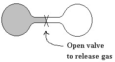The diagram on the left depicts an insulated, closed system consisting of two interconnected chambers separated by a valve. To start our thought experiment, we open the valve. Gas initially in the chamber on the left (shaded) expands adiabatically into the evacuated second chamber (adiabatic means no energy transfer between system and surroundings). The process is obviously spontaneous but energy is not involved. The gas has more room in the increased volume of the double bulb container. This increase in room allows more freedom of motion for the individual gas molecules. The driving force seems to be an increase in freedom of motion of the individual molecules. A given instantaneous combination of position and energy of all the molecules taken together is called a microstate. Clearly, there are more microstates available to the system if the gas expands into both chambers. Entropy is the scientific name for the macroscopic measure we use to evaluate these microstates of the system and is given the symbol $S$ .

The Second Law of Thermodynamics states:

For any spontaneous process in a closed system the entropy of the system must increase. ( $\Delta S_{sys} > 0$ )

or

For any spontaneous process (closed or not) the entropy of the universe must increase. ( $\Delta S_{universe} > 0$ )

The second law, thus, is a statement describing the driving force of all spontaneous processes. The tendency towards maximum entropy. We can see an analogy of this in our day to day lives in non scientific ways as well. Our rooms are rarely in perfect order unless we expend energy to keep it so. Without constant input of energy, the room would eventually be quite disorganized (this isn’t strictly the same thing but is an interesting parallel).

How do we measure entropy?

All processes have only two ways to transfer or change internal energy

work (organized energy)
heat (disorganized energy)

It seems reasonable that we can eliminate work as having anything to do with entropy as it merely represents the shifting of energy or matter from one location to another and that heat evolution or absorption must in some way be related to entropy changes.

We have, thus:

$\Delta S$ is proportional to heat transferred ( $q$ )

but $q$ is not a state function whereas we hope to make $\Delta S$ a state function. There are two things we can do to fix this problem.

Define $q_{rev}$ as the heat transferred for a reversible process (one which is done in infinitely small steps). Reversible simply means that at any step in the process, the system and universe both are essentially at equilibrium and hence the process can go forward or backwards with equal ease.

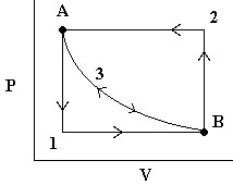
We can explore the idea of reversible energy transfer by considering the expansion and compression of an ideal gas in a cylinder where Temperature is always constant (isothermal):

Initially, we are at state A holding the gas in a volume $V_A$ in the cylinder with a pressure $P_A$ .

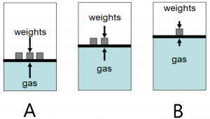
The image here shows three situations. State A, with heavy weights on the piston. This is a high pressure, low volume situation. State B is a low pressure, high volume situation and an intermediate state is shown as the weights are removed to move from A –> B or added to move from B –> A. The lengths of the arrows represent the pressures exerted by the weights (down) and by the gas (up) in the three diagrams.

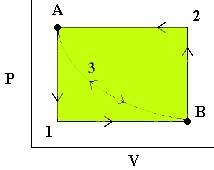
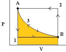
First, we release the pressure to $P_B$ . The gas quickly expands to a new volume $V_B$ . The $PV$ work done (by the system) is easily measurable as the area under curve 1 (in blue).
To reverse the process, we increase the pressure on the plunger back to $P_A$ and the gas then compresses back to $V_A$ . The work done (on the system) is the area under curve 2 (in green).
Note that the work done to compress the gas was more than the work done by the gas on the surroundings. Thus, we are loosing energy in this cyclic process.
Now consider the same process again but where we release the pressure infinitely slowly so that PV is always constant. In this case, we follow path 3 in either direction and we note that the work done on the environment by the system in the expansion phase is exactly the same as the work done by the environment on the system in the compression stage (yellow area). This is reversible work.

Note that at all times during the third process, the system and the universe are at equilibrium with each other. That’s because the process is occurring so slowly.

Since for any individual infinitesimal step, work $dw = -PdV$ . We must integrate this function over the range $V_1 \rightarrow V_2$ where $V_1$ is the volume at point A and $V_2$ is the volume at point B, i.e., we are finding the work done during the reversible expansion phase of the cycle. Of course, the work for the compression phase would be exactly the same magnitude but opposite in sign.

$w_{rev}= -\int_{V_1}^{V_2} P_{ex}dV$

[1]

Since we always have $P_{ex}$ @ $P_{gas}$ we can use the ideal gas law and write

$w_{rev} = - \int_{V_1}^{V_2} \frac{nRT}{V} dV = -nRT \int_{V_1}^{V_2} \frac{dV}{V} = -nRT \ln \frac{V_2}{V_1}$

[2]

Recall the relationship $P_1V_1 = P_2V_2$ , which leads to

$\frac{V_2}{V_1}= \frac{P_1}{P_2}$

This relationship allows us to rewrite equation [2] using pressures.

$w_{rev} =-nRT \ln \frac{P_1}{P_2} = nRT \ln \frac{P_2}{P_1}$

[3]

Since the expansions and compressions were done isothermally, the internal energy $U$ of the gas has not changed ( $\Delta U = 0 = q + w$ ) thus, we can write

$q_{rev} = -w_{rev}$

[4]

This function, although interesting is not a state function since the exact position of the reversible isothermal curve depends on the absolute temperature. Thus, to finally make the connection between S and q, we must factor out T, thereby creating a state function.

$dS = \frac{d q_{rev}}{T}$

[5]

or more generally, we must integrate between the initial and final state to get the overall change in entropy.

$dS = \int_{T_1}^{T_2} \frac{dq_{rev}}{T}$

[6]

For the isothermal reversible process we are discussing here, the integral simplifies to

$\Delta S = \frac{q_{rev}}{T}$

[7]

In order to evaluate this process, we will need to come up with the mathematical relationship for the energy transfer process. This relationship will depend on the exact situation we encounter.

Also note that this equation does not specify system or surroundings. If the work is done reversibly then it applies equally well for either. Since

$q_{rev,system} = -q_{rev,surroundings}$

[8]

It follows that

$\Delta S_{rev,sys} = -\Delta S_{rev,surroundings}.$

[9]

Hence,

$\Delta S_{rev,universe} = 0.$

[10]

In words, equation [10] tells us that there is no change
in the entropy of the universe for any process done reversibly.

Let’s use this new function under a variety of energy-transfer processes:

Examples.

Example 1:

A hot piece of metal at a temperature of 50.0°C is briefly placed in a tank of water at 15°C and then removed. While the metal is in the water, it loses 100. J of energy but neither the temperature of the metal, nor the water changed significantly. Calculate the entropy change of the metal, the water and the universe.

Since the temperature of the two objects didn’t change, we can use the simple equation $\Delta S = \frac{q}{T}$ to solve for the change in entropy of both the metal and the water. We know that 100 J of energy was exchanged between the metal and the water and it’s a negative value for the metal and positive for the water.

So,
Metal:

$\begin{array}{rcl} \Delta S_m &=& \frac{q}{T}\\ &=&\frac{-100\;\mathrm{J}}{(50.0+273.15)\;\mathrm{K}}\\ &=& -0.309\;\mathrm{J/K} \end{array}$

Water:

$\begin{array}{rcl} \Delta S_w &=& \frac{q}{T}\\ &=&\frac{+100\;\mathrm{J}}{(15.0+273.15)\;\mathrm{K}}\\ &=& 0.347\;\mathrm{J/K} \end{array}$

Finally, we add the two entropy changes to get the total entropy change (we are assuming nothing else changed).

$\Delta S_T = \Delta S_m + \Delta S_w = -.309 + .347 = 0.038 \mathrm{J/K}$

The entropy rose, which matches what we know about such a process whereby the heat leaves the hotter object and enters the cooler one.

Example 2:

Calculate the entropy change when two moles of an ideal gas expand isothermally so the pressure changes from 250.0 kPa to 100.0 kPa.

We Know the following three equations:

$w_{rev} = nRT ln\left(\frac{P_2}{P_1}\right),$

$q_{rev} = -w_{rev},$

and finally,

$\Delta S = \frac{q_{rev}}{T}.$

These three can be combined into a single equation:

$\begin{array}{rcl} \Delta S &=& -nR ln\left(\frac{P_2}{P_1}\right) \\ &=& -2\times 8.3145\; ln\frac{100.0}{250.0} = 15.24 J/K \end{array}$

The isothermal expanding of the ideal gas means it has more entropy.

Temperature change

We start with the derivative equation [5] we introduced above and we need to use the relationship heat. The simple calorimetry equation we learned earlier will work. For infinitesmal steps, $dq_{rev} = C\ dT$ so that we can complete the integral.

$dS = \frac{d q_{rev}}{T} = \frac{C\ dT}{T}$

[11]

Integrating we get

$\Delta S(T_1\rightarrow T_2) = \int_{T_1}^{T_2} \frac{C\ dT}{T} = C \ln \left( \frac{T_2}{T_1} \right)$

[12]

if we assume $C$ is constant. Equations [11] and [12] use $C$ as an overall heat capacity, referring to our total system. If we are using specific heat of a substance then we need to multiply by mass of that substance and if we’re using molar heat capacities we need to multiply by moles.

In general, $C$ is a function of temperature [ $= C(T)$ ] and this equation would need to be evaluated numerically. For our purposes, however, we’ll not bother with this complication. The assumption that $C$ is constant for relatively small temperature changes will give us satisfactory results.

15.2.1 Phase Transformation

A system undergoing a phase transformation is at equilibrium (the two phases are in equilibrium with each other). This is the same as saying that the energy is transferred reversibly between the system and the surroundings. Thus, the amount of energy transferred in a constant pressure situation, and thereby, also constant temperature is simply $q_{rev} = \Delta H$ . Thus, we can rewrite equation [7] above for any phase transition (fusion, vaporization, sublimation) as follows.

$\Delta S = \frac{\Delta H_{fusion}}{T_{fusion}}\qquad\qquad\Delta S = \frac{\Delta H_{vap}}{T_{vap}} \qquad\qquad\Delta S = \frac{\Delta H_{sublim}}{T_{sublim}}$

[13]

15.2.2 Isothermal Expansion/Compression of an Ideal Gas

For an Ideal gas isothermal process, we need to further develop the ideas we left. We combine equations [2], [4] and [7] to arrive at the following.

$\Delta S(V_1 \rightarrow V_2) = \frac{q_{rev}}{T} = \frac{nRT \ln \left(\tfrac{V_2}{V_1}\right)}{T}=nR\ln\left(\frac{V_2}{V_1}\right)$

[14]

or if we’re using the pressure (in this same gas PV change), we can combine equations [3], [4] and [7] to arrive at the following.

$\Delta S(P_1 \rightarrow P_2) = \frac{q_{rev}}{T} = \frac{-nRT \ln \left(\tfrac{P_2}{P_1}\right)}{T}=-nR\ln\left(\frac{P_2}{P_1}\right)$

[15]

Note that $\Delta S$ is often expressed as a molar quantity. If we are working with one mole quantities, then n = 1 and the equations [14] and [15] simplify slightly. Now we have all the tools necessary to calculate the entropy change for any non-chemical energy transfer process. With one more crucial piece of information, we can do more.

Third Law of Thermodynamics states:

The entropy of a pure crystalline material at absolute zero ( $0 K$ ) is zero.

Now we have all the tools necessary to calculate the absolute entropy for any pure material at any temperature (say, Standard Conditions). Hence, we can measure a standard entropy of a material $S^0$ (unlike the situation we saw earlier where we cannot define the absolute zero of enthalpy).

Thus, it is possible to tabulate lists of standard enthalpies for materials.

Examples:

A block of iron weighing 100.0 g is taken from a boiling water bath (NBP) and placed in an insulated container containing 100.0 g water at 0°C. Calculate The entropy change for the iron, the water and the whole process.

First, we define the system to be the iron and the water inside the insulated container. We recognize that the insulation means no heat is lost or gained

( $q_{total} = 0$ ). We also recognize that heat was moved within the system and because none was lost, we can state the following:

$\begin{array}{rcl} \textrm{Heat Transferred out of metal} & = & \textrm{heat transferred into water} \\ q_{Fe} & = & -q_{H_2O} \\ m_{Fe}C_{Fe}\Delta T_{Fe} & = & -m_{water}C_{water}\Delta T_{water} \\ m_{Fe}C_{Fe}[T_{Fe,final}-T_{Fe,initial}] & = & -m_{water}C_{water}[T_{water,final}-T_{water,initial}] \end{array}$

We will need to look up the heat capacities of the iron and of water. Since we are using gram amounts of iron and water, we look up the specific heats of the two.

C_Fe = 0.45 J K^-1g^-1; C_H₂O= 4.18 J K^-1g^-1

Note that the final temperature of the iron and the water will be the same so T_Fe,final = T_water,final; let’s call it T_f. so now we substitute these values to get

100.0 g × 0.45 J K^-1g^-1×{T_f – 100°C} = –100.0 g × 4.18 J K^-1g^-1{T_f – 0°C}

T_f = 9.7₁₉

The subscripted digits are written that way to help me keep track of the sig figs in this calculation. There are two sig figs so the number to be reported is 9.7. But, I would use 9.719 in any subsequent calculations to avoid round-off errors. Never round up intermediate answers.

Since we know the initial and the final temperature, we can use equation [12], modified for specific heats and mass measurements to determine the change in entropy.

$\Delta S =m C\; ln(\frac{T_2}{T_1})$

For iron:

$\Delta S = 100.0 g \times 0.45\mathrm{\; J K^{-1}g^{-1}}\;ln[\frac{273.15+9.719}{373.15}]$

$= -12.5\textrm{ J/K}$

For water:

$\Delta S = 100.0 g \times 4.19 J K^{-1}g^{-1}\;ln[\frac{273.15+9.719}{273.15}]$

$= 14.6\textrm{ J/K}$

$\Delta S_T = \Delta S_{iron} + \Delta S_{water} = -12.5 + 14.6 = +2.1 \textrm{J/K}$

Since the overall $\Delta S$ is positive the process is spontaneous.

Example: What is the entropy change for the vaporization of one mole of water at the NBP?

$\Delta S=\frac{\Delta H_{vap}}{T}=\frac{40650\; \mathrm{J}\;\mathrm{mol}^{-1}}{373.15\;\mathrm{K}} = 108.9\; \tfrac{\mathrm{J}}{\mathrm{K\; mol}}$

Back to Top

15.3 Standard Molar Entropies

The standard molar entropy of a substance is the entropy of one mole of that substance at Thermodynamic standard conditions (25°C, 1 bar, 1M conc,…)

We can always determine the absolute value for S° (J K^-1mol^-1) since we know the absolute zero of entropy (third law).

Appendix 5 lists S° values for many chemicals.

Since S is a state function, we can write the following:

ΔS = åS(final)- åS(initial)

[16]

For a chemical reaction at standard conditions, we can write

ΔS° = åS°(products)- åS°(reactants).

[17]

For example,

4 Fe(s) + 3 O₂(g) → 2 Fe₂O₃(s)

Δ $S$ ° = 2 $S$ °(Fe₂O₃) – {4 $S$ °(Fe) + 3 $S$ °(O₂)}

= 2(87.4 J/mol K) – 4(27.3 J/mol K) – 3(205.0 J/mol K)

= -549.4 J/mol K

NOTE 1: Large decrease in entropy is due to the fact that oxygen gas (reactant) becomes part of the solid iron oxide (product).

NOTE 2: This large decrease in entropy must be offset by a large release of enthalpy (exothermic) so as to increase the entropy of the surroundings to compensate for the loss of entropy in the system. I say “Must be” because the process of rusting is obviously spontaneous because our cars rust out so easily, yet the entropy change is negative. So enthalpy change is the only other component we can look at and it must be sufficiently exothermic that it overcomes the system’s negative entropy change by making the universe’s entropy change even more positive.

Note 3: This is actually a very common misconception of the second law that puzzles the un-initiated or uneducated. For example, life itself is an inherent negative entropy system (the body takes random items, food, oxygen from the air, etc. and creates the highly organized organism). Of course, the body, in growing gives off heat and thus creates even more increase in the surrounding’s entropy than the loss of entropy that develops within itself.

Another example

CaCO₃(s) → CaO(s) + CO₂(g)

Here we see that a gas is evolved and hence we expect that $\Delta S$ is positive.

$\begin{array} {rcl} \Delta S^{\circ} & = & S^{\circ}(CaO) + S^{\circ}(CO_2) - S^{\circ}(CaCO_3) \\ & = & (38.1\; J/mol\; K) + (213.7\; J/mol\; K) -(92.2\; J/mol\; K) \\ & = & 159.6\; J/mol\; K \;\;\;\;\; \end{array}$

$\Delta S$ is positive just like we predicted.

We see that as number of moles of gas increases, S increases and vise versa.

Back to Top

15.4 Gibbs Energy

Look at the rusting iron situation, we know it is spontaneous yet there is a decrease in system entropy.

We must consider the entropy change of the whole universe before we can explain for sure why the system will be spontaneous.

The measured value of enthalpy for the reaction

4 Fe(s) + 3 O₂(g) → 2 Fe₂O₃(s)

$\Delta H^{\circ} = -1648.4 kJ/mol$

We can thus calculate

$\Delta S^{\circ}_{surroundings} = \frac{-\Delta H^{\circ}_{system}}{T} = -\frac{-1648.4 kJ/mol}{298.15K} = + 5529 J/mol K$

Now, combining with the $\Delta S^{\circ}_{system}$ we just calculated, we get:

$\begin{array} {rcl} \Delta S^{\circ}_{universe} & = & \Delta S^{\circ}_{system} +\Delta S^{\circ}_{surroundings} \\ & = & -549.4\mathrm{ J/mol K} + 5529\mathrm{ J/mol K} \\ & = & 4980\mathrm{ J/mol K} \end{array}$

The entropy change of the universe is very large and positive despite the negative change of the system. This is a spontaneous reaction according to second law

So, we were able to calculate a parameter $\Delta S^{\circ}_{universe}$ that tells us definitively whether or not a system is at equilibrium. However, we would prefer to not be forced to deal with universe parameters if at all possible. Let’s rework the previous equation somewhat to try to incorporate only system thermodynamic quantities.

$\Delta S^{\circ}_{universe} = \Delta S^{\circ}_{system} + \Delta S^{\circ}_{surroundings}$	[18]
$\Delta S^{\circ}_{universe} = \Delta S^{\circ}_{system} + \frac{\Delta S^{\circ}_{system}}{T}$	[19]
$T\Delta S^{\circ}_{universe} = T\Delta S^{\circ}_{system} - \Delta H^{\circ}_{system}$	[20]

for sign consistency with enthalpy, we will multiply both sides by -1

$-T\Delta S^{\circ}_{universe} = -T\Delta S^{\circ}_{system} + \Delta H^{\circ}_{system}$

[21]

now, replace the left-hand side with a new parameter called the change in Gibbs Energy $\Delta G^{\circ}$ and rearrange the right-hand side. You will sometimes see this called “the change in Free energy”. Free energy is an old term is no longer being used in ‘up-to-date’ texts. Essentially, the energy is not “free”.

$\Delta G^{\circ} = \Delta H^{\circ} - T\Delta S^{\circ}$

[22]

Since these are all system parameters, we will drop the subscripts from now on.

The actual defining function for Gibbs Energy is

$G = H - TS$

[23]

but since we can’t actually measure the absolute enthalpy of a substance, neither can we measure the absolute Gibbs energy of a substance. Hence, this remains a defining equation only. It is not useful for any actual calculations or measurements we may wish to do.

We know that the second law states that the entropy of the universe must increase for any spontaneous process ( $\Delta S^{\circ}_{universe}$ is positive). Hence, $\Delta G^\circ}$
( $-T \Delta S^{\circ}_{universe}$ ) is negative.

We can now summarize:

$\begin{array}{rcl} \Delta G < 0 & \Rightarrow & \mathrm{spontaneous}\\ \Delta G = 0 & \Rightarrow & \mathrm{equilibrium}\\ \Delta G > 0 & \Rightarrow & \mathrm{non-spontaneous}\\ & & \textrm{(spontaneous in reverse direction)} \end{array}$

Let’s set up a table of the thermodynamic measurable for a reaction system and see what we can learn regarding system spontaneity.

case	ΔH	ΔS	ΔG	Spontaneous?
1	–	+	–	yes
2	–	–	– @ low T + @ high T	yes no
3	+	–	+	no
4	+	+	+ @ low T – @ high T	no yes

Since G is a state function (made up of H, T, and S which are each state functions) we can write

$\Delta G = \sum G(final) - \sum G(initial)$

[24]

For a chemical reaction at standard conditions, we can write

$\Delta G^{\circ} = \sum \Delta G_f^{\circ}(products) - \sum \Delta G_f^{\circ}(reactants).$

[25]

We must use Standard Gibbs Energy of Formation ( $\Delta_f G^{\circ}$ ) since we cannot define the absolute zero of Gibbs energy. This is exactly analogous with the case of Standard Enthalpy of Formation ( $\Delta_f H^{\circ}$ ). Note that we now have two ways to calculate $\Delta G^{\circ}$ . Equations [22] and [25] both allow us to determine a value for $\Delta G^{\circ}$ . The difference comes in the temperature factor that is explicit in [22]. Using [22], we can calculate Gibbs energy for any temperature (assuming $\Delta H^{\circ}$ and $\Delta S^{\circ}$ don’t change with temperature). However, equation [25] does not have temperature explicitly and so the value of $\Delta G^{\circ}$ we calculate using it will depend on the temperature at which the $\Delta_f G^{\circ}$ values were tabulated. Typically, that is 25℃.We will now do a few examples to familiarize ourselves with the calculations. For each of the following, calculate $\Delta G^{\circ}$ , $\Delta H^{\circ}$ and $\Delta S^{\circ}$ . The temperature in each of these examples is standard temperature (25℃).

a) CaCO₃(s) → CaO(s) + CO₂(g)

$\begin{array}{rcl} \Delta S^\circ & = & \sum S^\circ (products) - \sum S^\circ (reactants) \\ & = & S^\circ (CaO) + S^\circ (CO_2) - S^\circ (CaCO_3) \\ & = & 38.1\;\mathrm{ J/mol.K} + 213.7\;\mathrm{ J/mol.K} -92.4\;\mathrm{ J/mol.K}\\ & = & 158.9\;\mathrm{ J/mol.K}\\ \\ \Delta H^\circ & = & \sum\Delta_f H^\circ (products) - \sum\Delta_f H^\circ (reactants) \\ & = & \Delta_f H^\circ (CaO) + \Delta_f H^\circ (CO_2) - \Delta_f H^\circ (CaCO_3) \\ & = & -635.1\;\mathrm{ kJ/mol} + (-393.5\;\mathrm{ kJ/mol}) - (-1206.9\;\mathrm{ kJ/mol})\\ & = & 178.3\;\mathrm{ kJ/mol} \end{array}$

Gibbs-energy can now be calculated in one of two ways. We’ll do both here.

$\begin{array}{rcl} \Delta G^\circ & = & \Delta H^\circ - T\Delta S^\circ \\ & = & 178.3\;\mathrm{ kJ/mol} - 298.15\;\mathrm{K}\times (-0.1589\;\mathrm{ kJ/molK})\\ & = & 130.9\;\mathrm{ kJ/mol}\\ \\ & or\\ \\ \Delta G^\circ & = & \sum\Delta_f G^\circ (products) - \sum\Delta_f G^\circ (reactants) \\ & = & \Delta_f G^\circ (CaO) + \Delta_f G^\circ (CO_2) - \Delta_f G^\circ (CaCO_3) \\ & = & -603.5\;\textrm{kJ/mol} + (-394.4\;\textrm{kJ/mol}) - (-1128.8\;\textrm{kJ/mol})\\ & = & 130.9\;\textrm{kJ/mol} \end{array}$

Notice that either method of calculating $\Delta G$ gives the same value in this example, because the temperature was 298.15 K.

b) N₂(g) + 3H₂(g) → 2NH₃(g)

$\begin{array}{rcl} \Delta S^\circ & = & \sum S^\circ (products) - \sum S^\circ (reactants) \\ & = & 2\times S^\circ (NH_3) - S^\circ (N_2) - 3\times S^\circ (H_2) \\ & = & 2\times 192.7\;\textrm{ J/mol.K} - 191.5\;\textrm{ J/mol.K} - 3\times 130.6\;\textrm{ J/mol.K}\\ & = & -197.9\;\textrm{J/mol.K}\\ \\ \Delta H^\circ & = & \sum\Delta_f H^\circ (products) - \sum\Delta_f H^\circ (reactants) \\ & = & 2\times \Delta_f H^\circ (NH_3) - \Delta_f H^\circ (N_2) - 3\times \Delta_f H^\circ (H_2) \\ & = & 2\times (-45.9\;\textrm{ kJ/mol}) - (0) - (0)\\ & = & -91.8\;\textrm{kJ/mol} \end{array}$

Gibbs-energy can now be calculated in one of two ways. We’ll do both here.

$\begin{array}{rcl} \Delta G^\circ & = & \Delta H^\circ - T\Delta S^\circ \\ & = & -91.8\;\mathrm{kJ/mol} - 298.15\;\mathrm{K}\times (-0.1979\;\mathrm{kJ/molK})\\ & = & -32.8\;\mathrm{kJ/mol}\\ \\ & or\\ \\ \Delta G^\circ & = & \sum\Delta_f G^\circ (products) - \sum\Delta_f G^\circ (reactants) \\ & = & 2\times \Delta_f G^\circ (NH_3) - \Delta_f G^\circ (N_2) - 3\times \Delta_f G^\circ (H_2) \\ & = & 2\times (-16.4\;\mathrm{ kJ/mol}) - (0) - 3(0)\\ & = & -32.8\;\mathrm{ kJ/mol} \end{array}$

c) H₂(g) + Cl₂(g) → 2 HCl(g)

$\begin{array}{rcl} \Delta S^\circ & = & \sum S^\circ (products) - \sum S^\circ (reactants) \\ & = & 2\times S^\circ (HCl) - S^\circ (H_2) - S^\circ (Cl_2) \\ & = & 2\times 186.8\;\mathrm{ J/mol K} - 130.6\mathrm{ J/molK} - 233.0\mathrm{ J/molK}\\ & = & 20.0\;\mathrm{ J/molK}\\ \\ \Delta H^\circ & = & \sum\Delta_f H^\circ (products) - \sum\Delta_f H^\circ (reactants) \\ & = & 2\times \Delta_f H^\circ (HCl) - \Delta_f H^\circ (H_2) - \Delta_f H^\circ (Cl_2) \\ & = & 2\times (-92.3\;\mathrm{ kJ/mol}) - (0) - (0)\\ & = & -184.6\;\mathrm{ kJ/mol} \end{array}$

Gibbs-energy can now be calculated in one of two ways. We’ll do both here.

$\begin{array}{rcl} \Delta G^\circ & = & \Delta H^\circ - T\Delta S^\circ \\ & = & -184.6\;\mathrm{ kJ/mol} - 298.15\;\mathrm{K}\times (-0.0200\;\mathrm{ kJ/molK})\\ & = & -190.6\;\mathrm{ kJ/mol}\\ \\ & or\\ \\ \Delta G^\circ & = & \sum\Delta_f G^\circ (products) - \sum\Delta_f G^\circ (reactants) \\ & = & 2\times \Delta_f G^\circ (HCl) - \Delta_f G^\circ (H_2) - \Delta_f G^\circ (Cl_2) \\ & = & 2\times (-95.3\;\mathrm{ kJ/mol}) - (0) - (0)\\ & = & -190.6\;\mathrm{ kJ/mol} \end{array}$

In these cases, the two methods of determining ΔG° are equivalent. This is only true at standard temperature (298.15 K). In this case, you can choose the equation which best suits the data you have. If the temperature is not standard temperature then you have no choice but to use the first equation and to assume that ΔH° and DS° do not change with temperature. This assumption is not strictly true but is not a bad approximation for many cases.

We’ve seen that we can predict spontaneity of reactions using thermodynamic function ΔG. However, Thermodynamics gives us no information regarding the actual reaction path, specifically, how fast the reaction will occur. Hence, although Thermodynamics may predict that a reaction is spontaneous, it does not tell if the reaction will occur with any appreciable speed, if at all.

15.4.1 Temperature dependence of Gibbs Energy

Let’s explore the effect temperature has on ΔG. We’ve seen that equation [22]

$\Delta G^\circ & = & \Delta H^\circ - T\Delta S^\circ$

describes a temperature effect on G. This can be manifest in several ways.

At room temperature (25°C) the following is true (calculated previously)

CaCO₃(s) → CaO(s) + CO₂(g)

$\Delta S^\circ$ = 158.9 J/mol.K
$\Delta H^\circ$ = 178.3 kJ/mol
$\Delta G^\circ$ = 130.9 (non spontaneous)

Now, let’s try 1000 K

$\Delta G^\circ$ = 178.3 kJ/mol – 1000 K×158.9 J/mol.K = 19 kJ/mol

Now, let’s try 2000 K

$\Delta G^\circ$ = 178.3 kJ/mol – 2000 K×158.9 J/mol.K = –13 kJ/mol (it’s spontaneous at this temperature)

At what T would $\Delta G^\circ$ = 0?

0 kJ/mol = 178.3 kJ/mol –T×158.9 J/mol.K

T = 1122 K (849°C) the system is at equilibrium
(if all other conditions are held to standard conditions)

Note that all these values were considered to be Standard values of Gibbs Energy. Recall that 25ºC is not required for standard state, it is merely the temperature at which we normally tabulate these standard values.

15.4.2 Phase-Change Temperatures

We can also use equation [22] to calculate the phase-change temperature for any phase change since by definition, at that temperature, the two phases are in equilibrium with each other.

Thus, we can write

$\Delta_{phase-change}G^\circ = 0 = \Delta_{phase-change} H^\circ - T_{phase-change}\Delta_{phase-change} S^\circ$

$\therefore T_{ phase-change} = \frac{\Delta_{phase-change}H^\circ}{\Delta _{phase-change}S^\circ}$ .

[26]

For example, Let’s find the boiling point of water.

$\begin{array}{rcl} T_b(H_2O) & = & \frac{\Delta_v H^\circ(H_2O)}{\Delta_v S^\circ(H_2O)} \\ \\ & = & \frac{\Delta_f H^\circ(gas) - \Delta_f H^\circ(liquid)}{S^\circ(gas) - S^\circ(liquid)} \\ \\ & = & \frac{-242 - (-286)}{[189 - 70]/1000}\textrm{ K = 370 K} \end{array}$

That’s pretty close to the normal boiling point of 373 K. The discrepancy came in the assumption that the enthalpy change and the entropy change that we used (tabulated at room temp) was still valid at the normal boiling point of water. It was not a terrible assumption but clearly is was not perfect either.

15.4.3 Other dependencies of Gibbs Energy

We’ve seen that calculations of ΔG° are useful for predicting spontaneity of systems where all conditions are standard. Further, we explored the situation where the temperature is varied away from standard conditions. Now we will look into the more general case where other conditions are non-standard.

It is quite uncommon to deal with a reaction mixture, for example, where all concentrations are exactly 1 M. or with a gas-phase reaction where all partial pressures are 1 bar (100 kPa). In reality, we mostly deal with non-standard conditions of our reaction mixtures. How do we handle these?

We know that the sign of ΔG gives us information about the spontaneity of the reaction system (no superscript ° so not standard).

positive $\Rightarrow$ spontaneous to left

zero $\Rightarrow$ equilibrium

negative $\Rightarrow$ spontaneous to right

We also know that by comparing Q with K we can determine whether a reaction will be spontaneous or not

Q/K > 1 $\Rightarrow$ spontaneous to left

Q/K = 1 $\Rightarrow$ equilibrium

Q/K < 1 $\Rightarrow$ spontaneous to right

It turns out that these two functions are related (need the same kind of logic we saw in the earlier derivations at the start of this chapter)

Let’s begin our exploration using gas-phase reactions. We will quickly see that we can extend the results to cover all types of reactions.

Enthalpy changes in most system processes are relatively pressure independent. Therefore, we need only consider the effect pressure has on the entropy changes in a process to be able to understand how pressure affects the Gibbs-energy changes in that process.

S is relatively independent of pressure for solids and liquids but not for gases. For an ideal gas, what is the change in the value of G for as we move from standard pressure to non-standard? We will use equation [23] for the two states and subtract them.

$G-G^\circ = (H-H^\circ) - T(S-S^\circ)$

[28]

but since there is no concentration or pressure dependence for enthalpy, we know that (H-H°) = 0. Additionally, we can replace the (S– Sº) term using equation [15] where P₁ = Pº and P₂= P.

$G - G^\circ = RT ln\left( \frac{P}{P^\circ}\right)$

[29]

for one mole of gas or

$G = G^\circ + RT ln\left( \frac{P}{P^\circ}\right)$

[30]

NOTE 1: Many Texts write equation [30] as G = G° + RT ln (P), which is only correct if P is in units of bars (100 kPa)
since P° = 1 bar by definition. Any other units of pressure will result in the calculation of an incorrect value for G.

We recall that we already have a function which is called activity $(a = P/P^\circ)$ which we can use here. Thus,

$G = G^\circ + RT ln(a)$

We recall as well that since $a = 1$ for pure liquids and solids, this formula is not exclusive to gases.

As a special note, at this point, we should realize that Q is in fact more general than we’ve discussed here. we are using a = P/P° as the definition of activity. In fact, we can also define activities of solutes in solution in terms of concentrations as a = C/C°. This extension is perfectly analogous to the pressure case and the equation so derived is the same. Thus, we can write the general formula valid for all reactions as
$Q=\left(\frac{ \prod a_{products}}{\prod a_{reactants}}\right)$

Now consider a general chemical reaction

wA + xB → yC + zD

$\begin{array}{rcl} \Delta G & = & yG_C + zG_d - wG_A - xG_B \\ \\ & = & yG^\circ_C + zG^\circ_D - wG^\circ_A - xG^\circ_B \\ & & + RT [y\;ln(a_C) + z\;ln(a_D) - w\;ln(a_A) - x\;ln(a_B)] \\ \\ & = & yG^\circ_C + zG^\circ_D - wG^\circ_A - xG^\circ_B \\ & & +RT [lna_C^y + lna_D^z - lna_A^w - lna_B^x] \\ \\ & = & yG^\circ_C + zG^\circ_D - wG^\circ_A - xG^\circ_B + RT ln\left(\frac{a^y_C\;a^z_D}{a^w_A\;a^x_B}\right) \\ \\ & = & \Delta G^\circ + RT\;lnQ \end{array}$

The general (not necessarily standard-conditions) Gibbs energy change for this reaction is

$\Delta G = \Delta G^\circ + RT ln Q$

[31]

Note that the value for $\Delta G$ depends on the reaction conditions at the moment of measurement. The instant we allow the reaction proceed to any extent, $Q$ will change and hence, so too will $\Delta G$ . Thus, $\Delta G$ is not a constant of reaction. In fact, we could think of it as a slope of the $G$ versus reaction coordinate curve.

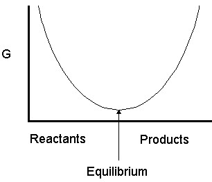
Note that when the slope of the
curve is down (negative) the reaction proceeds forward to equilibrium and
when it is up (positive) the reaction proceeds backwards towards
equilibrium. At equilibrium, the slope is zero.

At equilibrium, $Q = K$ and $\Delta G = 0$ , so we have

$0 = \Delta G^\circ + RT ln K$

[32]

or

$\Delta G^\circ = -RT ln K$

or

$ln K = - \frac{\Delta G^\circ}{RT}$

or

$K = \exp{\frac{-\Delta G^\circ}{RT}}$

[33]

Sometimes, we wish to calculate $\Delta G$ (non-standard) in circumstances where we do not know the thermodynamic data necessary to use equation [31] . In this case, we can get rid of $\Delta G^{\circ}$ by subtracting equations [31] – [32]

$\;\Delta G = \Delta G^\circ + RT ln Q$

$-\;[ 0 = \Delta G^\circ + RT ln K]$

to get

$\Delta G = RT ln Q - RT ln K$

$\Delta G = RT ln \frac{Q}{K}$

[34]

We now have a relation that can be used to determine Gibbs energy from equilibrium-type information and vice versa.

NOTE 1: The derivation shown above is only valid if we use relative activities to calculate our Q and K values. If we use concentrations in molarity and/or pressures in bars then we can safely use the equations in the boxes here since the standard values are 1 M and 1 bar. Thus, to convert from concentrations to activities by dividing by the standard leaves us with the same numbers if and only if we use these units.

We can use the above equations to calculate $K$ if we know $\Delta G^\circ$ , or vice versa,

N₂(g) + O₂(g) 2 NO(g)

$\begin{array}{rcl} \Delta G^\circ & = & 2\times \Delta_f G^\circ(NO) - \Delta_fG^\circ(N_2) - \Delta_fG^\circ(O_2)\\ & = & 2\times 86.2\;\mathrm{ kJ/mol}\\ & = & 173.2\;\mathrm{ kJ/mol} \\ \end{array}$

$\begin{array}{rcl} ln K & = & \frac{-\Delta G^\circ}{RT} = \frac{-173.2\mathrm{kJ/mol}}{8.314\mathrm{J/mol K}\times 298.15 K}\\ & = & -69.9\\ K& = & e^{-69.9} = 4.25 \times 10^{-31} \\ \end{array}$

Clearly, with a tiny $K$ value like that, the nitrogen in our air will not combine with the oxygen in or air to make nitrous oxide. Rather, any nitrous oxide we produce will tend to react back to nitrogen and oxygen, given enough time.

Example:

Calculate $\Delta G$ for the following reaction at room temperature

N₂(g) + 3 H₂(g) 2 NH₃(g)

if P_N₂ = 10. bar, P_H₂= 10. bar and P_NH₃ = 1.0 bar

$Q = \frac{a(\mathrm{NH_3})^2}{a(\mathrm{N_2})\times a(\mathrm{H_2})^3} = \frac{1^2}{10\times 10^3}=10^{-4}$

$K = 5.68\times 10^5 \textrm{(calculated earlier in notes)}$

$\Delta G = RT\;ln\left(\frac{Q}{K}\right) = 8.3145\textrm{ J/K} \times 298.25 \textrm{ K} \times ln\left(\frac{10^{-4}}{5.86\times 10^5}\right) =-55.7\textrm{ kJ/mol}$

at standard conditions we calculate

$\Delta G^{\circ} = -32.8\textrm{ kJ/mol}$

Hence, the stated conditions have a more negative $\Delta G$ than standard conditions, i.e., more spontaneous.

This difference in $\Delta G$ can be explained using Le Châtelier’s principle. We added more reactants to a system which tends to drive the reaction further to the right than standard conditions do. (more spontaneous)

NOTE: 1 bar = 100 kPa .

To convert from pressures in bars to activities, we simply drop the units since standard pressure is 1 bar (100 kPa).

Example:

Calculate $K$ for the following reaction at 700K:

C(s) + CO₂(g) 2 CO(g)

From thermodynamic data tables, we find the following:

$\begin{array}{|lccc|} \hline \textrm{Compound} & \begin{array}{c}\Delta_f H^\circ\\ \textrm{(kJ/mol)} \end{array} & \begin{array}{c}\Delta_f G^\circ\\ \textrm{(kJ/mol)}\end{array} & \begin{array}{c}S^\circ\\ \textrm{(kJ/mol)}\end{array}\\ \hline \textrm{C} & 0 & 0 & 6\\ \mathrm{CO_2(g)} & -393.5 & -394 & 214\\ \mathrm{CO(g)} & -110.5 & -137 & 198\\ \hline \end{array}$

$\begin{array}{rcl} \Delta H^\circ & = & 2(-110.5) - 0 - (-393.5) \\ & = & 172.5\;\mathrm{ kJ/mol} \\ \\ \Delta S^\circ & = & 2(198) - 6 - 214 \\ & = & 176\;\mathrm{ J/mol K}\\ \\ \Delta G^\circ & = & 2(-137)- 0 - (-394) \\ & = & 120\;\textrm{kJ/mol \;\;\;\;\;(this is only correct if T=298K)} \\ \\ So, use \\ \\ \Delta G^\circ &=& \Delta H^\circ - T \Delta S^\circ \\ &=& 172.5\;\mathrm{ kJ/mol} - 700\mathrm{ K} \times 176\;\mathrm{ J/mol K} \\ &=& 49.3\;\textrm{ kJ/mol (valid at 700 K. All other conditions are std state)}\\ \\ Finally:\\ K&=& \exp \left(\frac{-\Delta G^\circ}{RT}\right)\\ &=& \exp \left(\frac{-49.3\;\mathrm{ kJ/mol}}{8.3145\;\mathrm{J/mol K} \times 700\;\mathrm{ K}}\right)\\ &=& 2.1\times 10^{-4} \end{array}$

Remember that $\Delta H^\circ$ and $\Delta S^\circ$ are assumed to be constant over the temperature range (298 K – 700 K). This is not strictly true. $\Delta G^\circ$ has been somewhat ‘corrected’ for temperature. In this case, the ‘ $^\circ$ ‘ symbol on the $\Delta G^\circ$ implies that all other conditions but temperature are standard state
(poor symbology).

We can also use these ideas to be able to develop an expression which can give us an equilibrium constant at any temperature if we know $\Delta H^{\circ}$ and $\Delta S^{\circ}$ and $K$ at some other temperature.

We start from equation [32] and then expand it using equation [22].

$ln K = -\frac{\Delta G^\circ}{RT}$

Sub in $\Delta G^{\circ} = \Delta H^{\circ} - T\Delta S^{\circ}$

$ln K = -\frac{\Delta H^\circ}{RT}\ + \frac{\Delta S^\circ}{R}$

We know $K_1$ at $T_1$ and wish to find out $K_2$ at $T_2$ .

We can write for temperatures $T_1$ and $T_2$ the following two cases:

$ln K_2 = -\frac{\Delta H^\circ}{RT_2}\ + \frac{\Delta S^\circ}{R}$ (2)

$ln K_1 = -\frac{\Delta H^\circ}{RT_1}\ + \frac{\Delta S^\circ}{R}$ (1)

now subtract case (1) from (2) to get the following

$ln\left(\frac{K_2}{K_1}\right)=-\frac{\Delta H^\circ}{R}\left(\frac{1}{T_2}-\frac{1}{T_1}\right)$

[34]

This is the van’t Hoff equation, which we have already seen earlier in this course. It assumes again that $\Delta H^{\circ}$ is constant with temperature. We can use this equation to quickly tell the effect of $T$ on $K$ .

Consider an exothermic reaction ( $\Delta H^{\circ}$ is negative). What will happen to $K$ as the temperature is increased? Looking at the right-hand side (RHS) of the equation, if $T_2 > T_1$ the RHS will be negative. This means that (on the LHS) the argument to the natural logarithm function must be less than one, i.e., $K_2 < K_1$ . Hence, as $T$ ↑, $K$ ↓ for an exothermic reaction.

Examples

$\Delta G$ can be thought of as the ‘maximum’ amount of work which can be obtained from a spontaneous process at constant T and P.

$w_{max} = -\Delta G$

Consider the oxidation of glucose:

C₆H₁₂O₆(s) + 6 O₂(g) 6 CO₂(g) + 6 H₂O(l)

$\Delta H^\circ = -2808$ kJ/mol $\Delta G^\circ = -2870$ kJ/mol

Now consider a person of 60 kg climbing a 100 m high hill. How much glucose will they need to consume to obtain sufficient energy for the climb.

$w = mgh = 60\textrm{ kg} \times 9.8\textrm{ ms}^{-2} \times 100\textrm{ m} = 60\mathrm{ kJ}$

we’re only interested in the magnitude of energy used, so we’ll drop the minus sign from the Gibbs energy value.

$60\textrm{ kJ} \times \frac{1\mathrm{ mol}}{2870\textrm{ kJ}}\times \frac{180\textrm{ g}}{1\textrm{ mol}} = 3.8 \textrm{ g of glucose}$

This means the person needs 3.8g of glucrose if 100% of energy released from oxidation of glucose is used in climbing. Assuming, of course that 100% of the food energy is converted into climbing work.

Actually, The only way one can achieve 100% efficiency is if the waste heat from the system is absorbed by a heat sink at absolute zero (0 K).

Murphy’s version of the laws of thermodynamics

You can never win, you can only break even.
You can only break even at absolute zero.
You can never reach absolute zero.

15.5 Coupled Reactions

Sometimes, we can use spontaneous reactions to drive non-spontaneous ones in the direction we desire.

Consider the following reaction
$\begin{array}{|l|l|} \hline & \Delta H^\circ = +79.5\;\mathrm{kY/mol}\\ \mathrm{Cu_2S(s)} \rightleftarrows} \mathrm{2\;Cu(s) + S(s)} & \Delta S^\circ = -22.4\;\mathrm{J/mol.K}\\ &i.e.,\; \Delta G \textrm{ is positive at all temperatures}\\ & \Delta G^\circ = +86.2\;\mathrmkJ/mol}\\ \hline \end{array}$

Copper ore is most often found in the form of Cu₂S. Copper is one of the earliest metals to ever have been smelted. Clearly, the process can not happen if it’s just the pure copper ore that is being heated (or cooled) because the reaction is non spontaneous at any temperature. If we couple this reaction with a highly spontaneous one, we can make the overall process proceed spontaneously.

$\begin{array}{l|ll} \\ \mathrm{S(s) + O_2(g) \rightleftarrows SO_2(s)} & \Delta H^\circ = -296.8\;\mathrm{kJ/mol} & \Delta G^\circ = -300\;\mathrm{kJ/mol}\\ \\ \mathrm{Cu_2S(s) \rightleftarrows 2 Cu(s) + S(s)}&\Delta H^\circ = +79.5\;\mathrm{kJ/mol} & \Delta G^\circ = +86.2\;\mathrm{kJ/mol}\\ \\ \hline \\ \mathrm{Cu_2S(s) + O_2(g) \rightleftarrows 2 Cu(s) + SO_2(g)}&\Delta H^\circ = -217.3\;\mathrm{kJ/mol} & \Delta G^\circ = -213.2\;\mathrm{kJ/mol}\\ \\ \end{array}$
Now, the overall reaction is both exothermic and spontaneous. Early humans likely discovered copper metal when they used rocks with the ore in them as their camp-fire rocks. There was plenty of oxygen being drawn into the process by the heat of the camp fire and the high temperatures would have accelerated the process of smelting the copper out. It still would have taken a pretty observant person to notice the tiny droplets of copper and realize they were made from the blue stones and that they could be useful.

In biological reactions, we talk about food as fuel and and we breath oxygen which is used with the fuel to produce energy and leave behind CO₂ . Clearly, this cannot be happening at standard conditions as a simple combustion reaction. Our bodies could not survive that kind of high temperatures. Instead, we use intermediate reactions that add up to the overall combustion but in which any individual step is small enough that it does not heat up the cells too much. The ADP $\rightleftarrows$ ATP reversible reaction is coupled with any process which needs to be forced. The reaction is:

ATP^3- + H₂O $\rightleftarrows$ ADP^2- + H₂PO₄^–
$\Delta G^\circ = -30\textrm{ kJ/mol},\;\;\; \Delta H^\circ = -20\textrm{ kJ/mol},\;\;\; \Delta S^\circ = +34\textrm{ J/mol.K}$

Thus, in biological systems no compound can be created which requires more than 30 kJ of energy for one mole of any given reaction step in the synthesis process. This is one of the biggest single limiting factors in the diversity of life on the planet.

For some extra practice, try these problems. Thermo Problems

License

Icon for the Creative Commons Attribution-NonCommercial-ShareAlike 4.0 International License

15.1 Spontaneous Processes

Back to Top

15.2 Entropy and the Second law of Thermodynamics

Examples.

Temperature change

15.2.1 Phase Transformation

15.2.2 Isothermal Expansion/Compression of an Ideal Gas

Back to Top

15.3 Standard Molar Entropies

Back to Top

15.4 Gibbs Energy

15.4.1 Temperature dependence of Gibbs Energy

15.4.2 Phase-Change Temperatures

15.4.3 Other dependencies of Gibbs Energy

Examples

15.5 Coupled Reactions

License

Share This Book