19 Appendix 8: Atomic orbitals.
The overall atomic orbital for any one electron can be symbolized as  . This function incorporates all the features we discussed when talking spherical harmonics. The function can be written as a product of two parts. The function can be written in Cartesian space
  as we are familiar with but a mathematically simpler way to write it is in polar coordinates,
  . In this polar coordinate space, we can still represent the full 3d space but now, any nodes that depend on the radius (spherical shaped nodes) can be expressed as simply the value of
  where the functions crosses zero. similarly, by expressing the wave functions in polar coordinates, we will be using sines and cosines of those angles. Since sines and cosines cross zero, we will have the angular notes described. The relation ship between polar coordinates and Cartesian coordinates can be seen in the following diagram.
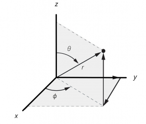 and polar coordinates
  . The variable represents the radial distance from the nucleus (at the origin of the axes). The variable
  is the angle from the z axis and the variable
  is the angle from the
  axis to the projection of the vector into the
  plane. You can convert from polar coordinates to Cartesian coordinates using the following equations,
![\[x = r\; sin \theta\; cos \phi\]](https://ecampusontario.pressbooks.pub/app/uploads/quicklatex/quicklatex.com-648f2b14069229ae6bde8890df4d4c52_l3.png "Rendered by QuickLaTeX.com")
![\[y = r\; sin \theta\; sin \phi\]](https://ecampusontario.pressbooks.pub/app/uploads/quicklatex/quicklatex.com-068ba77b1c954d1a1e9292257c8a445b_l3.png "Rendered by QuickLaTeX.com")
![\[z = r\; cos \theta\]](https://ecampusontario.pressbooks.pub/app/uploads/quicklatex/quicklatex.com-462dd50f714c78dfcc99567bfe9068ab_l3.png "Rendered by QuickLaTeX.com")
So, we can write the atomic orbital in terms of cartesian coordinates  or in polar coordinates
  . Now that we have the function in polar coordinates, we can rewrite the overall wave function as the product of two functions, a radial part
  shows how the functions vary with the distance, , from the nucleus and the angular part
  shows how the function varies with angles and
  .
.
![\[\Psi(r,\theta,\phi) = R(r) \times Y(\theta,\phi)\]](https://ecampusontario.pressbooks.pub/app/uploads/quicklatex/quicklatex.com-d6bd3d0dd96bc4a1ee3528c762a52b85_l3.png "Rendered by QuickLaTeX.com")
This is actually a common mathematical technique called separation of variables. It allows us in this case to more easily visualize how the functions vary with radius (the radial function) and with angle (the angular function). The functions tend to zero as the radial distance tends to zero. That is represented in the reverse exponential part of the radial function for any orbital. You will see something like  in all the radial functions. This is a generic reverse exponential where the value goes to zero as goes to infinity.
![\[\linespread{2} \begin{array}{ll} Angular\; Part\; Y(\theta,\phi) & Radial\; Part\; R_{n,l}(r)\\[2pt] \hline\\ Y(s) = \left(\frac{1}{4\pi} \right)^{1/2} & R(1s) = 2\left( \frac{Z}{a_0}\right)^{3/2} e^{-\sigma/2}\\[4pt] & R(2s) = \frac{1}{2\sqrt{2}}\left(\frac{Z}{a_0} \right)^{3/2}(2-\sigma)e^{-\sigma/2}\\[4pt] & R(3s) = \frac{1}{9\sqrt{3}}\left(\frac{Z}{a_0} \right)^{3/2}(6-6\sigma+\sigma^2)e^{-\sigma/2}\\[8pt] Y(p_x) = \left(\frac{3}{4\pi}\right)^{1/2}sin\theta\; cos\phi & R(2p) = \frac{1}{2\sqrt{6}}\left(\frac{Z}{a_0}\right)^{3/2}\sigma e^{-\sigma/2}\\[4pt] Y(p_y) = \left(\frac{3}{4\pi}\right)^{1/2}sin\theta\; sin\phi & R(3p) = \frac{1}{9\sqrt{6}}\left(\frac{Z}{a_0}\right)^{3/2}(4-\sigma) e^{-\sigma/2}\\[4pt] Y(p_z) = \left(\frac{3}{4\pi}\right)^{1/2}cos\theta &\\[8pt] Y(d_{z^2}) = \left(\frac{5}{16\pi}\right)^{1/2}(3\;cos^2\theta -1) & R(3d) = \frac{1}{9\sqrt{30}}\left(\frac{Z}{a_0}\right)^{3/2}\sigma^2 e^{-\sigma/2}\\[6pt] Y(d_{x^2-y^2}) = \left(\frac{15}{16\pi}\right)^{1/2} sin^2\theta\; cos 2\phi\\[6pt] Y(d_{xy}) = \left(\frac{15}{16\pi}\right)^{1/2} sin^2\theta\; sin 2\phi\\[6pt] Y(d_{xz}) = \left(\frac{15}{16\pi}\right)^{1/2} sin\theta\; cos \theta\; cos\phi\\[6pt] Y(d_{yz}) = \left(\frac{15}{16\pi}\right)^{1/2} sin\theta\; cos \theta\; sin\phi\\ \end{array}<span style="font-size: 1em">\]](https://ecampusontario.pressbooks.pub/app/uploads/quicklatex/quicklatex.com-b3dc3c93372de9c53f60d569188c0438_l3.png "Rendered by QuickLaTeX.com")
Note: 
That table looks a bit daunting at first glance but with a bit of thought, it is not that hard to understand. The first take-a-way is that those orbitals are simply math functions. They don’t have anything in them that is truly incomprehensible. Let’s look at a few examples and see how these equations work.
Consider the 1s orbital. 
Notice that there is only one angular function  for all
  orbitals. it is simply a constant. there is no angular dependence for an orbital. All orbitals are spherical. Notice the radial part of the function. It has two parts. The constant in front of the exponential
  and the exponential decay part
  . The constant in front, along with the constant in the angular part together are called the normalization factor. This is to make sure the orbital is exactly the right size to hole 1 electron. When integrated over 3-space, the result is 1, i.e., one electron exactly fits in each orbital. The exponential decay, as described above means the orbital tends to zero as the distance from the nucleus becomes zero. If you square the wave function, you will get the electron probability function. So another way of saying this is as the radial distance increases to infinity, the probability of finding the electron goes to zero.
 ).
).2s orbital
Now, let’s consider a slightly more complicated orbital, a  orbital. This one has
  so there are no radial nodes (remember, quantum number
  is the number of angular nodes), that means the one node in the
  orbital must be radial (spherical). We expect to see the function go through zero and change phase at a certain distance (at the node). Looking at the radial part of the function, you see some constants again, which we can ignore as just part of normalization. You can see the exponential decay term just as you saw in the
  orbital. What’s new is the parenthetical term
  . This term will make the whole function go to zero when
  . Now look at the simulation of the orbital.
 orbital. The colours represent the phase of the orbital. the red is one phase and the green is the opposite. At the boundary between the two colours, you can see the spherical node. This would occur at the distance
  according to the table of orbital functions listed above.
So, we can make up any orbital we want by combining the correct combination of angular and radial parts from the table above.
2pz orbital
Let’s make an orbital with an angular node rather than a radial node. The  function is the simplest orbital that has an angular node. Let’s make a
  function; you make it by multiplying the
  angular with the
  radial part.
![\[\Psi(p_z) = \left(\frac{3}{4\pi}\right)^{1/2}cos\theta \times \left(\frac{3}{4\pi}\right)^{1/2}cos\theta}\]](https://ecampusontario.pressbooks.pub/app/uploads/quicklatex/quicklatex.com-ae7fa13882ce896aed4270b38468390c_l3.png "Rendered by QuickLaTeX.com")
Note that the radial part has only the exponential decay part. There are no parts of this radial function that go to zero. The angular part of the  function has a
  in it; anywhere that is zero, the whole function will go to zero. Since the cosine function passes through zero at
  (aka 90°), this means the node will be in the plane. Look at this projection of the orbital, looking down the axis with the
  axis vertical.
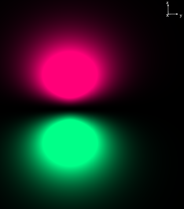
 orbital. Notice that the axis is vertical in this view. the node is in the plane so the lobes are along the axis. the colours represent the phase of the orbital so the boundary where the phase changes is the node, the plane. This is horizontal in this image.
So, we have seen a radial node and an angular nodes and seen the functions that have defined them in our math. We can imagine that any orbital can be described using this kind of function, except that as the number of nodes increases, the math would get more complicated.
3d(xy) orbital
Let’s try something a bit more complicated; a  function. Notice that all the 3d functions have the same radial part, so we just choose the correct angular part and multiply it to the radial part.
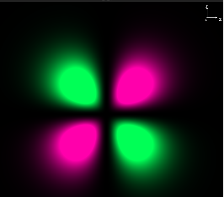 orbitial. you are looking down the axis, the
  axis is vertical and the x axis is horizontal. The nodes are planar, there are two of them (
 means 2 nodes;
  means they are both angular). One is in the
  plane and the other is in the zx plane.
This orbital, like all the others has a normalization constant. It tails off to zero as the distance goes to infinity. But this one has angular nodes. there are sine and cosine functions and you know that these pass through zero once as you go around the unit circle. The particular combination of angular functions in the 3d(xy) orbital gives us this shape. Note that there are no left-over spherical nodes; n=3 means 2 nodes. means they are both angular (planar in this case).
3pz orbital
OK, One last orbital. This one also with two nodes. So it must be an function. This one has one angular node (so  ; a p orbital) and one radial node. This function will look similar to the 2p function above but you will also be able to see the radial node in addition to the angular planar node.
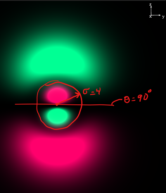
 orbital. It is projected in the same orientation as the orbital above. Notice, just like in the orbital above, there is a planar node in the xy plane. In addition to that angular node, you can easily see a radial node that is centered on the nucleus. This radial node occurs at a distance of
  according to the function table above and it cuts the two lobes of the p into smaller parts making a kind of mushroom topped shape. I have drawn (free-hand) the two nodes in red for you to visualize easier. Notice, the colour changes each time you cross one of the nodes. That indicates that the phase changes when you cross the nodes. In black/white drawings, we often use “+” and “−” instead of colours to represent the two phases.
Finally, to make up the entire wave function for a multi-electron atom, you would multiply one complete orbital for each electron in the atom into an overall wave function for the entire atom.
In theory, you would be able to do this for multi-atomic species, multiplying all the atomic orbitals on all the atoms together, with proper adjustments of the normalization factors, to make new molecular orbitals. But that is a process for an upper-year class.
Once you have a wave function for your species, you use the Schrödinger equation to get out the array of energies  .
.
 .
.
