7 Molecular Structure
Michael Mombourquette
7.1: Lewis Dot Structures
One of the early questions asked by scientists, once the concepts of atoms and molecules had been firmly established was “How are Atoms Bonded?” We’ve developed many theories over the years in attempts to explain the bonding between atoms in various substances. In some substances, our models explain the bonding that holds the atoms and molecules to each other quite well but as we explored more and more deeply, we have always been able to find examples of substances where the models don’t work. We will explore here, the development of models and the uses and limits to the models as we work through better and better models.
There are many different types of materials with properties that vary widely. Yet even the simplest of models can be useful.
For example, Salt, NaCl, liquid molecules, H2O, gaseous molecules, H2 and Cl2?
We say that there is a chemical bond between the atoms involved
Chemical Bonds: → Forces that hold together atoms in a molecule.
Lewis Electron Dot Symbols Convenient for explaining chemical bonds. Very simple, theory but can be quite a useful visualization tool.
Recall the concept of the atomic core. We will assume that the inner (core) electrons in a molecule are not involved in chemical bonding since they are held tightly to the nucleus and are not involved in either electron sharing or electron transfer processes. As a result, Lewis Dot diagrams display only the outer or valence electrons.
OCTET RULE: In compound formation an atom tends to gain or lose electrons or to share electrons until there are eight electrons in its outer shell. (Often but not always the valence shell).
7.1.1: Normal Valence State
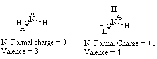
Valence is used for many purposes. The only usage I will give it is Valence = number of atoms that are bonded to an atom. For example, Oxygen displays its valence of 2 in the compound H2O while nitrogen with a valence of 3 forms NH3. The valence of the elements can be equated to the number of unpaired electrons on the atom. However, we must notice that the ground state of some of the elements (Be, B, C) is not the same as the valence state. In other words, the element in free space in its minimum energy configuration (ground state) is not necessarily the same as the element in a molecule.
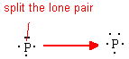
To reconfigure an atom into its ‘normal valence’ state, we can split the non-bonding pair (lone pair) of electrons into two unpaired electrons. In the case of Be, we split the two 2s electrons into two unpaired electrons (into orbitals not necessarily called 2s and 2p but we’ll get to that later).
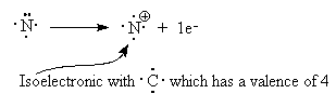
Similarly, we can expand the valence of B and C by splitting their lone pairs into single electrons. In each of these cases, we increase the “valence” by 2 for each lone pair we split up. We can do this because there are a maximum of 4 orbitals at the n=2 quantum level into which we can put electrons with minimal expense energy-wise. If we tried to split the lone pair on Nitrogen into two unpaired electrons we would run into the limit of the number of orbitals. N, has only 4 orbitals (places) to hold electrons. The normal ground state of N already has at least 1 electron in each of the four orbitals. If we tried splitting the lone pair we would have no place to put the extra electron without moving it to an n=3 orbital. That would cost too much energy.
The energy we pay to move electrons around to form their normal valence state is returned to us when we form bonds. We don’t want to have to pay too much to move electrons around because the energy returns when we form a bond may not compensate. That’s another story we’ll discuss later.
We see that this simple way of representing the valence electrons around the atom can actually help us understand the observed ‘valence’ of the atoms. NOTE that the valence indicated is an exact match with the number of unpaired electrons in the Lewis valence state structure. We will use this concept of valence to build our Lewis Dot Structures. Make sure you memorize (at least the last line of) this table!
| Table of Valences | ||||||||
|---|---|---|---|---|---|---|---|---|
| Group | 1 | 2 | 3 | 4 | 5 | 6 | 7 | 8 |
| #Valence e– | 1 | 2 | 3 | 4 | 5 | 6 | 7 | 8 |
| Valence | 1 | 2 | 3 | 4 | 3 | 2 | 1 | 0 |
| Lewis Dots Groundstate |
Li · | Be : | : B· | · C : · |
· : N · · |
· : O : · |
·· : F : · |
·· : Ne : ·· |
| Lewis Dots normal valence state |
Li · | · Be · | · · B · |
· · C · · |
· : N · · |
· : O : · |
·· : F : · |
·· : Ne : ·· |
7.1.2: Ionic Bonds
In an ionic bond, one atom loses all its outer electrons (leaving behind a filled inner shell) while another atom gains electron(s) to fill its valence shell. The two ions attract each other according to Coulombic interactions.
For example, consider sodium chloride.
![]()
The Lewis Structure for the Salt NaCl, shows two ions which have their (Now) outer shells of electrons filled with a complete octet. In the case of the sodium cation, the filled shell is the outermost of the ‘core’ electron shells. In the Chloride ion, the outer shell of valence electrons is complete with 8 electrons. The two ions are bonded with ionic bonds.
Consider the compound magnesium oxide: MgO.
![]()
Note that in both cases, the positive ions are metals and the negative ions are non-metals. This is generally true for ionic compounds.
In general Metals have lower ionization energies and form cations.
Non metals have high ionization energies (and high electron affinities and form anions.
| 1 | 2 | 3 | 4 | 5 | 6 | 7 |
| Li+ | Ba2+ | |||||
| Na+ | Mg2+ | Al3+ | ||||
| K+ | Ca2+ | |||||
| Rb+ | Sr2+ | |||||
| Cs+ | Ba2+ |
7.1.3: Covalent Bonds
Covalent bonds involving the sharing of electrons to form ‘bonding pairs’ of electrons and satisfy their normal valences. It turns out that when this is done, most commonly, there are eight electrons around each atom. This is the so-called octet rule.
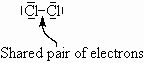
Take Cl2. Each Cl atom has one unpaired electron ![]() . It is unlikely that an ionic type bond has formed since the two atoms are identical and such a transfer would leave one chlorine with only 6 electrons. More likely, they share a pair of electrons so that each can ‘think’ it has 8 electrons in its valence shell. Note that Cl is below F in the periodic table and so has a normal valence of 1 with three extra lone pairs.
. It is unlikely that an ionic type bond has formed since the two atoms are identical and such a transfer would leave one chlorine with only 6 electrons. More likely, they share a pair of electrons so that each can ‘think’ it has 8 electrons in its valence shell. Note that Cl is below F in the periodic table and so has a normal valence of 1 with three extra lone pairs.
Mostly, this type of bonding occurs between non-metal atoms.
Consider PCl3:
![]()
Note: I hid the lone pairs on the chlorines to emphasize the electron configuration around the phosphorous.
The normal valence of P (like N) is 3 with one lone pair. So, when combined with three Cl atoms, the structure as drawn above satisfies this valence requirement. The P shares one of its unpaired electrons with each of the three Cl atoms to form three covalent bonds. We see the normal valence of P = 3 and of Cl = 1 is satisfied with this structure. All four atoms now have a completed octet.
It is not always necessary to use two dots to represent the pair of electrons. A dash can also represent the pair of electrons, especially in bonds. Consider the following examples
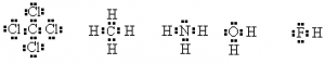
or using a — to represent a bonding pair
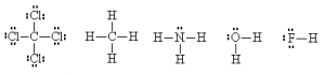
It is sometimes even possible to simplify even further by hiding the outer electrons on the outside atoms (but not the ‘central’ one), as long as this doesn’t cause ambiguities. One can also use a dash alongside the atom to represent lone pairs.
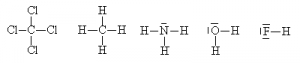
This method is quicker to draw, more clearly shows that electron pairs are bonding pairs and helps distinguish the bonding pairs from the non-bonding pairs more easily. It is also possible to use the dashes to represent both the bonding pairs and the non-bonding pairs of electrons. This is also an acceptable way of doing a Lewis dot structure for some purposes.
There are exceptions to the Octet rule. For example, H has only a 1s orbital occupied. The other orbitals are all higher in energy and not involved in the chemistry of hydrogen.
Consider water H2O.
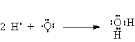
There are only two electrons in the valence shell of hydrogen but that’s all it takes to fill the first shell. Hence, the octet rule doesn’t apply.
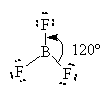
Other compounds where the Octet rule is not obeyed include some Boron compounds.
Boron has only three unpaired electrons to share. It has a normal valence of 3 with no lone pairs according to the table of valences.
![]()
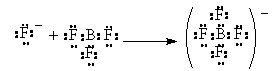
Here, Boron has only 6 valence electrons. It cannot complete its octet and remain a neutral compound. BF3 can combine with an F– ion to complete its octet as follows.
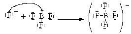
One of the lone pairs on the fluoride is shared with the boron and forms a bond.
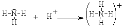
The ammonium ion is another example of a complex ion that fills the octet rule. In this case, the nitrogen in ammonia has a completed octet but it combines with the hydrogen ion, which has an empty 1s orbital. In this case, the bonding pair of electrons comes completely from the nitrogen. The positive hydrogen ion is attracted to and then shares the (originally) non-bonding pair of electrons on the N to form a covalent bonding pair.

These polyatomic ions can form ionic compounds such as NH4+Cl– and Na+BF4–.
7.1.4: Expanded/Hyper-Valences
Elements in row 3,4,… have access to d orbitals (unlike row 2 elements that have only s and p orbitals) and can therefore have more than 8 electrons around them in certain compounds. Recall that P has a normal valence of 3 with one lone pair. If that lone pair is divided into two extra unpaired electrons to be used in creating bonds, we then have a hypervalence of 5.
By expanding the valence of P, we change it from Valence=3 with one lone pair to Valence=5 with no lone pairs. PCl5 is one such compound that has P with a hypervalence of 5 and no lone pairs.

Here, we see that the valence of P is 5. Since this is higher than its normal valence, we call it the hypervalence. (hyper means higher than).
Other elements, like S can have more than one hypervalence. S has a normal valence of 2 with two lone pairs. If we split the lone pairs one at a time to create extra unpaired electrons for bonding, we can create hypervalences of 4 and 6. We can see these at work in the following series of compounds. SF2, SF4, and SF6. Try drawing these Lewis structures out, Note that the number of lone pairs on the S decreases by one as the valence goes up by 2.
At one time, it was believed that the octet rule was the overriding factor in determining bonding. Using this logic, it was once thought that the Noble gases (He, Ne, …) were totally unreactive since they already have a filled octet. Using the concept of hypervalences, we see that we can expect that some noble-gas compounds can form. We have in recent years produced compounds of Xe as follows:
XeF2, XeF4, and XeF6, XeO4. All four of these compounds are using a hypervalent state of the Xenon since its normal valence is zero.
What possible valence states might you expect for iodine, bonded to one or more fluorines? Is one of them a normal valence state?
The results of these expansions can be summarized in the table below.
| Table of Normal and Hypervalences | |||
|---|---|---|---|
| Elements | Valence | lone pairs | Example |
| P, As, Sb… | Normal 3 | 1 | |
| 5 | 0 | ||
| S, Se, Te, … | Normal 2 | 2 | |
| 4 | 1 | ||
| 6 | 0 | ||
| Cl, Br, I, At… | Normal 1 | 3 | |
| 3 | 2 | ||
| 5 | 1 | ||
| 7 | 0 | ||
| Ar, Kr, Xe, Rn… | Normal 0 | 4 | |
| 2 | 3 | ||
| 4 | 2 | ||
| 6 | 1 | ||
| 8 | 0 | ||
A more compact view of this same table could be drawn like the following table. There, are listed the valences and where applicable, the number of lone pairs. for example, the fifth column normal valence has a 3,1 representing 3 bonds and 1 lone pair. Notice that hypervalent states only occur where atoms have extra electrons in lone pairs that can be split up to make extra bonding sites. This requires d orbitals and is therefore restricted to the n > 3 valence levels.
| Table of Normal Valences and Hypervalences | ||||||||
|---|---|---|---|---|---|---|---|---|
| Group | 1 | 2 | 3 | 4 | 5 | 6 | 7 | 8 |
| Normal Valence states | 1 | 2 | 3 | 4 | 3,1 | 2,2 | 1,3 | 0,4 |
| Hyper-valent states | 5,0 | 4,1 | 3,2 | 2,3 | ||||
| 6,0 | 5,1 | 4,2 | ||||||
| 7,0 | 6,1 | |||||||
| 8,0 | ||||||||
7.1.5: Multiple Bonds
Some compounds have more than one pair of electrons shared by two atoms.
Since one pair of shared electrons is a bond, two pairs would be two bonds, etc. The number of bonds joining any two atoms is called the bond-order.
Take CO2, for example. The normal valence of the C is 4 and the normal valence of O is 2. The only way we can connect these three atoms together in a way that satisfies both their valences is to connect them as follows. Recall from the table of valences that C, in its normal valence state has 4 bonds and no lone pairs and O has 2 bonds and 2 lone pairs so that’s the way we draw them in the Lewis structure.
![]()
The C=O bond order is 2
Now try C2H4. Again, the normal valences of C (=4) and H (=1) can be satisfied with the following structure.

The C=C bond order is 2 whereas the C-H bond orders are all 1.
Now compare C2H2 and N2 (they’re isoelectronic). Here again, the normal valences of all the atoms is satisfied, only by creating multiple bonds. Note that according to the table of valences that N has one lone pair.
![]()
7.1.6: Formal Charge and Oxidation Number
There are several ways of accounting for electrons when we create these structures. We’ve seen that in the case of NaCl that the ‘bonding’ pair of electrons is completely on the chloride anion and hence, completely removed from the sodium cation. On the other hand, in Cl2, the bonding pair is exactly shared between the two identical chlorine atoms.
These represent two extremes of chemical bond formation. Most compounds form bonds which lie somewhere in between these two extremes, neither 100% covalent nor 100% ionic in nature.
However, for the purposes of bookkeeping, we need to make assumptions about the nature of the bonds. We will either assume 100% covalent or 100% ionic when we do the counting.
Oxidation Number
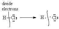
There is an alternate way to count electrons on molecules. This results in a different individual number for each atom than we got using formal charges but like formal charges, the sum of these oxidation numbers must always add up to the overall charge on the species. To count oxidation numbers, we assume 100% ionic bonding where electrons are completely transferred from the less electronegative atom to the more electronegative atom. For example, even though HCl is not ionic bonded, we make that assumption for the sake of accounting. (governments do it all the time when they make up new budgets)
![]()
In the case of HCl, Cl is more electronegative than H so it takes both electrons. Thus, to determine the oxidation number of the two atoms, we count the electrons differently.
(Higher electronegativity)
Oxidation # = Core Charge – # non-bonded electrons – # bonded electrons
(Lower electronegativity)
Oxidation # = Core Charge – # non-bonded electrons.
Thus, we can now determine the Ox#’s for HCl.
Oxidation # of Cl (more electronegative) = 7 – 6 – 2 = -1
Oxidation # of H (less electronegative) = 1 – 0 = +1
Notice that both the formal charge and the oxidation number of an atom is reported like a charge. Don’t make the mistake of thinking that they really are charges. They are merely the result of the particular accounting method chosen.
Oxidation numbers will be revisited when we take up Oxidation/Reduction chemistry later.
Formal Charge
For the purposes of discussing covalent bonding and stability of molecules, we will do our accounting assuming that all bonds are 100% covalent, i.e., all bonding pairs of electrons are shared equally between the bonded atoms. Thus, in the molecule H-Cl, one electron from the bond is counted as belonging to the H and the other to the Cl.
 |
| Half of the electrons in the bonding pairs go to one atom and the other half go to the other atom. |
Recall that these structures ignore the core electrons. Hence, in our calculations of charge (either formal charge or oxidation number) we must do the same. So, to calculate the formal charge of the H and the Cl in HCl, we must first determine the core charge and then subtract from that the number of electrons in the outer shell (after the division).
More precisely,
Formal Charge = Core Charge – # non-bonded electrons – 1/2 # bonded electrons.
For hydrogen, the core charge is the atomic number Z = 1 since there are no inner electrons. Recall that the Core charge is the column number of the periodic table (discounting the transition metals).
Hence,
Formal charge of H = 1 – 0 (non-bonded electrons) – 1/2 ×2 (bonded electrons) = 0
Similarly,
Core Charge of Cl = 17 – 10 = 7
Formal charge of Cl = 7 – 6(non-bonded electrons) – 1/2 ×2 (bonded electrons) = 0
The Shortcut:
Most experienced chemists do not use the preceding equations. They use their knowledge of the periodic table and experience to develop these numbers without calculating. Here’s how they do it.
- The formal charge of any atom in its normal valence state (or hypervalence state) is always zero. So, if you were able to recognise that the Cl and the H were both in their normal valence states then you could have quickly stated that their formal charges were both zero.
- If the element is not in its normal valence state (and not in a hypervalence state) then by comparison with neighbouring atom valence states, you can assign a formal charge.
Look at NH4+. The nitrogen in this molecule (we’ve seen the Lewis structure above) has a valence state that seems to look like C. It has a valence of 4 with no lone pairs. Since C is one to the left of N in the periodic table, we assign a formal charge of +1 to the N since C has one less electron than N. We verify that this structure is correct since the sum of all the formal charges must add up to the charge on the species.
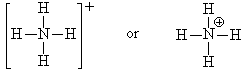
When we draw the Lewis structure, we may indicate that the N has the formal charge of +1 by a plus sign in a circle next to the N.
Note that the number of bonds formed by an atom is related to its formal charge.
For example, the normal valence (number of bonds) of N is 3 but with a formal charge of +1, it can actually form 4 bonds.
You could think of it as
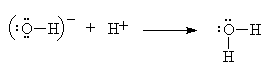
Now try OH–. Again, we note that there is a charge of -1 on the species. When we join these two atoms together, we can only have one bond between the O and the H since H has a valence of 1. Now O looks like F which has a valence of 1 with 3 lone pairs. F is one atom to the right so we assign a formal charge of -1 to the Oxygen since F has one more electron than O.
![]()
We know that we’re correct since the sum of the formal charges equals the total charge.
7.1.7: Using Formal Charges in Lewis Structures
For the our purposes, we will use formal charges to help us determine the best Lewis structure of covalent compounds (and covalently bonded polyatomic ions). It is important to keep the formal charges as low as possible. Real molecules are not very stable if they have high localized charges. Our modeling should reflect this. If you use a structure that gives you a formal charge of more than +1 then you have the wrong structure.
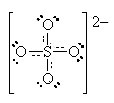
Let’s look at SO42- as an example. Lets try out several different models and eliminate all but the correct one using our rules as we know them so far.
 In this first attempt we’ve met the normal valence of all the oxygens so they all have a formal charge of 0. The S looks like one of the configurations of noble gas (valence of 8 with no lone pairs). Since the noble gases are two columns to the right, that gives a formal charge of -2 on the S. The sum of the formal charges adds up to the overall charge but there’s a high charge on S which would not be stable.
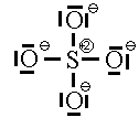 In this second model, we can see that there is only 1 bond between the S and each O. This makes the S look like a column 4 element (two columns to the left) and we assign a +2 formal charge and it makes the O atoms all look like F so we put 3 lone pairs and a formal charge of -1. The sum of the formal charges adds up to the overall charge so we’ve put the correct number of electrons but there’s a high charge on the S.
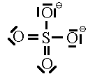 If we move to satisfy the normal valence of two of the oxygens and the S by making double bonds to two of the O atoms we get the structure shown on the right. This time, two of the oxygens and the S are all in a normal (or hyper-) valence state so have a formal charge of zero. Two of the oxygens still look like F and so have a formal charge of -1. The sum of the formal charges adds up to -2 which is the overall charge. Thus, this structure works and it has the lowest formal charges of the three models we’ve tried here.
A good final check is to count the electrons in your structure and see if they add up to the sum of the valence electrons and the charge.
Count the electrons:
    S:  6
   4O: 24
Charge  2
total  32
Sulfate has 32 valence electrons that are paired up in 16 pairs. Count the bars in our diagram representing pairs of electrons (either bonding or non-bonding) and we see 16 electron pairs are indeed drawn in on the diagram. We have done a good Lewis-Dot structure.
The one problem left is that this model seems to make two of the oxygens different from the other two. Experiment doesn’t agree with this prediction. We’ll see later how we modify the model to accommodate this.
We’ll see later an even greater reason for the stability of this molecule.
7.1.8: Summary of the Rules
So far, we’ve been exposed to the rules of creating Lewis structures one at a time. Let’s summarize here the rules we’ve learned so far.
- Draw the structure of the species trying first to satisfy the normal or hypervalences of the elements.
- If you must use a valence that is not a normal (or hyper-) valence for that particular atom then assign formal charges to the atoms based on comparison with the valence states of atoms from neighbouring columns in the periodic table.
- If the formal charge on any one atom has a magnitude greater than 1 then try to rearrange pairs of electrons to lower the formal charges, keeping in mind the valence states as in step 2.
- Sum up the formal charges. They must equal the overall charge on the species. If not, your structure is wrong, start again.
- Assign lone pairs as a needed to make the atoms look like one of the images in the table of normal and hypervalences. Thus, an atom with 3 bonds needs looks like N and so needs 1 lone pair (unless it is in group 3), etc.
- If you can create more than one structure, the one with the smallest formal charges is the best one.
With practice, these rules become simply intuitive and you will see that eventually you will be able to quickly draw Lewis structures without reference to them any further.
Try using these rules to create Lewis structures for the following: CO32-, O2, AlCl3, IF3, XeF6. (Check here for the answers)
For a numeric, method to find a Lewis structure, click here.
As one last example, let’s look at Carbon monoxide and work its Lewis Structure out using the rules.
Since we have only two atoms, they must be bonded to each other and (with filled octets) they must be configured the same.
___________________________
If we try to make the atoms look like C we would come up with the incorrect structure shown here.
![]()
Here, the C looks OK, it has 4 bonds and no lone pairs, just like the table of valences describes so it has a formal charge of zero. The Oxygen, of course, also has 4 bonds on it, just like C which is two columns to the left so O has a formal charge of +2. The overall +2 charge says that we have 2 too few electrons in this model of what should be neutral carbon monoxide.
___________________________
Next, we try to satisfy the normal valence state of O. Again, an incorrect result:
![]()
This time, the O is neutral but the C has a -2 charge on it. This model has 2 too many electrons on it, since carbon monoxide is a neutral molecule. We can write off this picture too.
___________________________
So, we were unable to come up with a model where the normal valence states of either atoms is satisfied. Perhaps, if we “split the difference”…
![]()
This is the only Lewis structure that has a sum of formal charges that add up to zero, the charge on the molecule. This one looks strange but is the only correct Lewis dot structure.
However, the Lewis-dot model does not properly predict atomic charges here. In this final model, we see that both the C and the O have a charge and that, in fact, the charges seem opposite of what we might have expected considering that O is very electronegative, compared to C. In all likelihood, the O will pull the three bonding pairs closer to it, making an unevenly shared triple bond with most of the negative charge closer to the O. That will bring the actual atomic charge closer to zero for each atom.
Remember, the Formal charge is not necessarily the real charge. It is just the results of a very simple model for keeping track of electrons.
7.1.9: Special Cases
Radicals
There are some few exceptions to the rules which may cause us trouble. These are the radicals, In radicals, there is an odd number of electrons so no matter how many models we try where all the electrons are paired up, we’ll never be able to make the model match the real molecule. One such examples of this is NO2. If we add up the electrons on this species, there are 5 from the N and 6 each from the two Os for a total of 17 electrons. An odd number. Now, pretend we didn’t do that. We don’t know that we cannot use the normal rules to make a Lewis structure that will work. Let’s see what trouble we might get into.
| 1. | In this first model, we’ve satisfied the normal valence of one O and the N but one of the O atoms looks like F and we must give it a charge of -1. Obviously wrong since the NO2 molecule is neutral. | |
| 2. | Here, we see a second attempt. This time, we find that the oxygens are both in their normal valence state and that there’s a + charge on the N. This doesn’t work either. | |
| 3. | 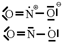 |
Finally, we’ve given up trying to use pairs of electrons. We note that model 1 seems to have 1 electron too many. By removing one electron from the N or from the O of model 1, we arrive at a structure whose formal charge adds up to the overall charge of zero. Now the question is:Which of these is the correct one. You can’t tell. This is the point where our rules for Lewis structures break down and we realize we need something better.
The latter of these has the lower formal charges so we might suspect that it is the favoured one. However, EPR experimental data puts the unpaired electron almost exclusively on the N as shown in the former of the two.
|
Resonance
Many molecules have electrons that are localized in simple orbitals (bonds, lone pairs, etc.) and exist at room temperature primarily in their ground state. Such species are often well represented using a single Lewis dot structure. However, many molecules or ions have electrons that either are not localized in one position or perhaps where higher energy levels are easily reachable at room temperature. These species may not be so well represented by a single Lewis dot structure because the species itself does not stay in one configuration.
Lewis dot diagrams give us a static picture of what the molecule or ion might look like. So how do we deal with situations were a static model does not tell us the entire story. We assume that we can represent each different configuration by a Lewis dot structure and in some cases, all these different diagrams add to our overall understanding of the real species.
There are two different ways that we might find multiple Lewis dot structures:
- Lewis dot diagrams displaying higher than optimal formal charges represent higher energy states of the species.
- There may be several ways to draw the optimal configuration Lewis dot diagram, which could mean that the ground-state electrons are not fixed into local orbitals.
We will restrict our discussion here to situations where we can find more than one equivalent ground-state Lewis structure. In these cases, we must consider whether the multiple Lewis dot structures represent chemically different species or different electronic configurations of the same species. In our sulphate ion case, there are six identical structures and they an interchange one for the other as indicated below. (We use a single double-headed arrow to represent movement of electrons only. We assume Atoms do not move because they are several thousand times more massive and hence several thousand times slower than electrons)
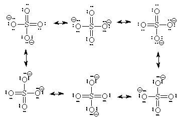
Since there are six structures which interchange on a rapid basis, we need to rethink our ideas of formal charges and of Bond order.
In this case, we can define average formal charge for any one atom to be:
![\[Avg\; FC = \frac{\mbox{Sum of Formal Charges on an atom in all resonance structures}}{\mbox{Number of structures}}\]](https://ecampusontario.pressbooks.pub/app/uploads/quicklatex/quicklatex.com-4cff07616fc4ed7dbe5aff363ed0a6e4_l3.png "Rendered by QuickLaTeX.com")
Hence, for the top oxygen (pretend we have nailed down the ion so it can’t rotate. That way we can keep track of the motion of the electron within the ion.) going clockwise, starting with the top-left structure we get:
![\[Avg\; FC = \frac{0 + 0 + 0 + (-1) + (-1) + (-1)}{6} = \frac{-3}{6} = -1/2\]](https://ecampusontario.pressbooks.pub/app/uploads/quicklatex/quicklatex.com-29242d13bed91def93a8c734bf54ed52_l3.png "Rendered by QuickLaTeX.com")
The Avg. FC for the Sulphur, is obviously zero since it is so in all the structures.
We can also define an average bond order (BO) for any pair of atoms as:
![\[Avg\; BO = \frac{\mbox{Total number of bonds between atom pair in all resonance structures}}{\mbox{Number of structures}}\]](https://ecampusontario.pressbooks.pub/app/uploads/quicklatex/quicklatex.com-408a2a030f88e4c6dc1ae8ffe3131b44_l3.png "Rendered by QuickLaTeX.com")
Thus, for the pair SO (top) we can calculate as before
![\[Avg\; BO = \frac{2 + 2 + 2 + 1 + 1 + 1}{6} = \frac{9}{6}\mathrm{ = 1 1/2}\]](https://ecampusontario.pressbooks.pub/app/uploads/quicklatex/quicklatex.com-1ed44d92edbd972d6a50d5515b1ec5eb_l3.png "Rendered by QuickLaTeX.com")
The calculated average bond order of 1 1/2 implies that there is always 1 bond joining the SO pair and half the time, there is a second bond joining that same pair (according to this resonance structures model). Hence, the solid and the dotted lines joining the pair in the final “average” diagram.
_____________________
Some people will also argue that higher energy structures must be included in the list of possible resonance structures. We saw two such structures already for the sulphate ion.

These two Lewis dot structures (*and some other higher-charged ones) do have the correct number of electrons (sum of the formal charge equals the overall charge) but for reasons (discussed above), we determined that they do not represent the lowest possible energy configuration. In the purest view, they are also possible resonance structures but they represent higher energy configurations of the sulphate ion. Since the high-energy configurations do not last long (first law of thermodynamics), they don’t contribute as much to the overall picture as do configurations represented by the six ground-state Lewis dot diagrams above. So, we will not count the high-energy diagrams in the calculations of average bond order or formal charge.
Electron-Deficient Resonant Structures
In the previous example as in most resonance structures you will encounter, the average bond order is greater than one for the bonds where the resonance is actually occurring. That is because, typically, one bond remains in place throughout the resonance process and a second (or third) bond moves from place to place in the different resonant structures.
In certain special situations, where there are insufficient electrons for normal bonding to occur, resonant structures can be formed between atoms of a species to form a bond order that is actually less than one. In these cases, there must be at least one of the series of resonance structures where the bond is completely missing. Obviously, these compounds would not be as stable as those we normally think of as having resonance but they do exist.
Take the molecule B2H6. It does exist but if we try to draw a normal Lewis-dot structure, we cannot find a way to bond all the atoms together at one time. Using resonance structures we show how the bonds can move in such a way as to create a bond for at least part of the time.
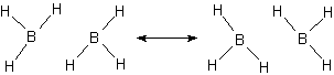
In this resonance model, we see that the B–H bond order to the central hydrogens is actually only 1/2, i.e., the bond exists only half the time in this picture. An average picture that shows the entire structure as being connected might be
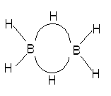
Here, we see that the central hydrogens are bridging between two borons in a curved, electron-deficient 3-centre bond sometimes called a banana bond. This three-center bond has only two electrons in it and hence the bond order of the individual B−H portions of this have a bond order of only 1/2.
Molecules with this kind of bonding are stable mostly in boron compounds although there are examples of other three-center electron deficient bonds. It is possible to create valid Lewis structure models of such bonding in any analogous compound made up of column 3 elements like Al, Ga, In, Tl. We can draw the analogous structures but for other reasons, beyond the scope of this discussion, actual chemical analogues such as Al2H6 or Ga2H6 are not as stable and if created, some of these would quickly reform into other, more stable compounds. We can find other examples of electron-deficient three-center bonds that are stable and analogous to the B2H4molecule, for example, Al2Cl4 exists, is stable and used electron-deficient three-center bonds that are quite analogous to those shown above.
Lewis Bases and Lewis Acids
We can now use the ideas developed here to describe a process where a bond is formed when a species with an extra electron pair forms a covalent bond with a species which is deficient in an electron pair.
This obvious acid-base reaction is exactly analogous to the reaction between ammonia and the hydrogen cation.
In this reaction, still would refer to the ammonia as a base and the hydrogen cation as the acid, but how about the following

In this case, the F– ion has the extra electron pair and uses it to bond with the BF3 in which the B is missing one electron pair to complete the octet. The Fluoride ion donates an electron pair to the Boron. The Fluoride acts just like the ammonia or the hydroxide ion did in the previous two examples where they clearly the base. Thus, the electron-pair donor is a Lewis Base. The electron pair Acceptor is the Lewis Acid (NOTE there is a typo in the book p. 240)
Hydrogen Bonding
One last type of bond can be explained now using the Lewis dot structures. It is very similar in concept to the Lewis-acid/Lewis-base bond formation. In this case, however, a bond is not formed, merely a strong attraction.
This type of bond can only form between a hydrogen (which is bonded to a very small high-electronegative atom like N, O, or F) and some other electronegative atom (N, O, F) in which there are non-bonded electron pairs available.
In water, for example, the oxygen is bonded to two hydrogens but has two non-bonded electron pairs available to it. Hence, the H from one molecule may be able to join to the lone-pair of electrons from the O of a different molecule.

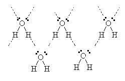
Hence, the molecules of water are attracted to each other strongly because of the phenomenon called Hydrogen bonding.
This explains the unusually high boiling point of water when compared to other molecules of similar molar mass such as CH4 which is a gas well below room temperature. It also explains the fact that ice floats. When crystals of ice form, the hydrogen bonding forces the molecules into a regular arrangement which is in fact spaced out further than when the molecules are in the liquid phase. Hence, ice is less dense than water and it floats.
7.2: VSEPR Intro
Experimental evidence clearly shows us that the Lewis Model of molecular bonding, while having its merits, is far from complete. Take for example the molecule Chlorofluoromethane (CH2FCl) If we draw the Lewis Dot Structure for this molecule, we get one of two possibilities:
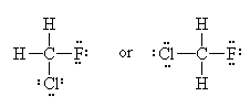 =>
=>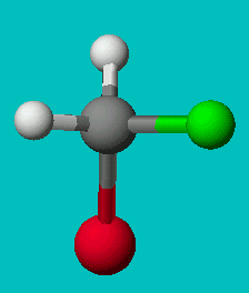 or
or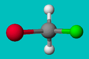
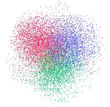
If you’re good at visualizing, you can clearly see that the two molecules depicted here are identical (Cl is red, F is green). They are superimposable. If you’re not so good at visualizing, try to rotate these two models with your mouse to make them identical.
These structures seem to show that there are two different versions of this molecule, one in which the chlorine is adjacent to the fluorine and one where it is across from it. Experimental evidence shows us that there is only one molecule with the formula CH2FCl, despite there being two different ways to depict the molecule using only Lewis dot theory.
Using similar logic, we see that the molecule CHFClBr has two distinct forms and experiment shows them to have different physical properties (optical properties). So, there are clearly examples where the Lewis dot theory breaks down. There must be further theories that can explain these observations.
It turns out that the flat representations produced in the Basic Lewis structures are the problem. Molecules are not generally flat but exist in three dimensions.
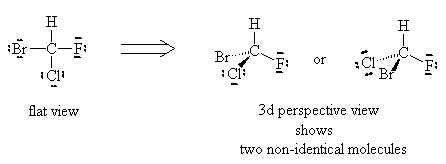
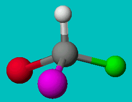 or
or 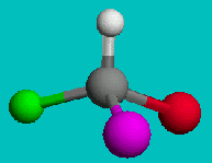
Can you superimpose these? You’ll find it is impossible to line them up. If you line up two elements the other two will be reversed, no matter which way you try. These two molecules are not superimposable, even though they have the exact same formula. They are called enantiomers or optical isomers.
7.2.1 VSEPR geometries
The Valence Shell Electron Pair Repulsion Theory (VSEPR), as it is traditionally called helps us to understand the 3d structure of molecules. Although we will speak often of electron pairs in this discussion, the same logic will hold true for single electrons in orbitals, and for double bonds, where one could think of the bond as consisting of two pairs of electrons. In general, the region in space occupied by the pair of electrons can be termed the domain of the electron pair. The domain is related to the orbitals we have discussed earlier (and will elaborate on later) but the two do not necessarily refer to the same thing.
7.2.2: Basic Geometries
The general concept is that the pairs of electrons repel each other and wish to locate themselves as far as possible from each other about a given nucleus. Hence, for two pairs of electrons on a nucleus, the two pairs would locate themselves exactly opposite each other, forming a bond angle of exactly 180°. If three pairs exist, they will locate themselves in a plain about the nucleus at angles of 120° from each other. higher numbers of electrons form 3d arrangements as follows.
Table: Geometry and Electron Pair Arrangements. The angles given are the ideal angles for such an arrangements.
| Electron Pairs | e– pair (domain) Geometry | e– pair diagram |
|---|---|---|
| 2 | Linear |  |
| 3 | Trigonal planar | 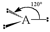 |
| 4 | Tetrahedral | 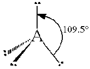 |
| 5 | Trigonal bipyramidal | 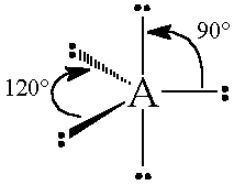 |
| 6 | Octahedral | 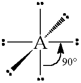 |
7.2.3: Expand geometry lists
We’ll now go through a set of example molecules and/or ions and discuss their geometries. It is important to note that the shape of the molecules as we discuss them here is not always the same as the electron domain geometries described above.
We will consider the molecular shapes, starting with the simplest and working up to the more complicated examples. In addition, I’ll mention a classification system which may be helpful in counting electron domains used herein.
- The classification system follows:
- A represents a central atom (any atom being considered. It need not actually be the centre of the molecule)
X represents an atom bonded to A. It could be single, double or triple bonded. It makes no difference to the scheme.
E represents a non-bonded electron domain (lone pair).
For example, methane CH4 is an AX4 molecule while ammonia NH3 is an AX3E molecule. Both of these molecules have four electron domains and hence would have a tetrahedral domain geometry as listed above. However, the shape of the molecules are not the same as we will see below.
2 pairs of electrons
BeCl2 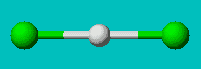
| AX2 | LINEAR |
This molecule is linear. The Be does not fill its octet shell in this situation. To do so would put a large negative charge on it and a positive charge on the Chlorine atoms. This would simply not happen since Cl is so much more electronegative than Be.
3 pairs of electrons
BF3 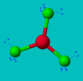
| AX3 | Trigonal Planar shape |
4 electron pairs
CH4 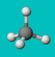

| AX4 | tetrahedral |
NH3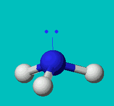

| AX3E | trigonal pyramidal |
H2O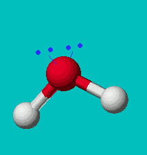

| AX2E2 | bent or angular |
HF 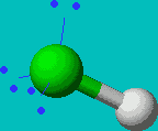

| AX1E3 or just AXE3 |
linear |
Note that in all these cases, the electron-domain geometry is tetrahedral. However, the molecular shape is not always so. In the case of CH4, the molecule is actually tetrahedral in shape with a perfect Tetrahedral angle of 109.5°. The next two examples have lone pairs which occupy a larger domain volume (push more on the bonding pairs) and reduce the bond angle to less than 109.5°. The last case, HF, is simply a liner diatomic molecule. There is no bond angle.
5 electron pairs
PCl5 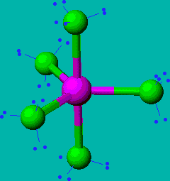

| AX5 | trigonal bipyramidal |
SF4 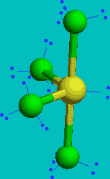

| AX4E | See Saw or disphenoidal |
ClF3

| AX3E2 | T-shaped |
XeF2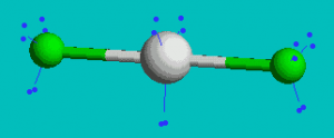
 AX2E3 Linear
In these cases, the electron-domain geometry is always trigonal bipyramidal. However, only the first molecule is that shape with the ideal angles of 90° and 120° for the axial and equatorial bonds, respectively.
In the case of SF4, there is one lone pair and four bonding pairs. The lone pair will preferentially locate itself in an equatorial position since that position has only two other pairs of electrons within 90° while an axial position would have three. Thus, the molecular would be see-saw shaped or the more technically correct name, disphenoidal. The bond angles would be less than the ideal angles of 90° and 120°.
ClF3 has two lone pairs and they both locate themselves in equatorial positions for the same reasons as described in the previous case. This molecule is T-shaped with bond angles of less than 90°.
6 electron pairs
SF6 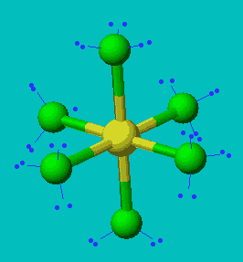

| AX6 | Octahedral |
ClF5 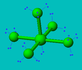

| AX5E | Square Pyramidal |
XeF4 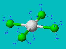 |

| AX4E2 | Square Planar |
In all these cases, the electron-domain geometry is octahedral and in the case of SF6, so is the shape. The molecule ClF5 has one lone pair and five bonding pairs but since all positions in the octahedral geometry are equivalent, it doesn’t matter which position the lone pair takes. I drew it on the bottom position here for visual effect. In the case of XeF4, the two lone pairs will locate themselves on opposite sides of the square planar molecule. In the case of the XeF4 molecule, the lone pairs will orient themselves in a square plane and the molecule will be linear in shape.
7.3:Bonding
There are two different basic models that Chemists use when describing bonding in molecules. The one they choose depends on their purpose. These are Valence bond theory and Molecular orbital theory. We will look at each in turn. Keep them separate in your mind. Students regularly mixup these two in their attempt to understand things like hybridization, etc.
7.3.1: Valence Bond Theory
This is the simpler of the two models. Valence Bond (VB) theory uses localized orbitals. that means that each orbital is fixed in position and cannot spread out over the whole molecule. A bond is simply made by overlapping two atomic orbitals, one from each of the two bonded atoms.
Normal Basis set atomic orbitals
So far, we’ve seen that we can explain some experimentally observed properties using simple models like Lewis Dot structure and VSEPR. These models still do not explain many chemical properties. In this section, we will develop a new model that explains further some of the chemical reactivities we observe and also ties in our knowledge of atomic orbitals and expands it further.
So far, we’ve been saying that molecular bonding involves atomic orbitals in some way. We will now explore atomic orbitals and develop an understanding of their involvement in molecular orbitals (e.g. bonds).
Lets look at the VSEPR models identify the places where they are lacking in explanations. We’ll then look at the model of localized orbitals and see how this new model is better.
To make a bond, we must use an atomic orbital from each atom involved in the bond. What do these atomic orbitals look like?
In the molecule BeCl2 ![]() , we saw that there are two electron domains on opposite sides of the beryllium atom involved in the bonds to the two chlorines. How do these domains arise? Our atom of beryllium has atomic orbitals for its valence shell (n = 2) of type s and p. If we try to make bonds using two of these orbitals, we find that we cannot come up with two orbitals that are identical and have lobes on opposite sides of the Be.
, we saw that there are two electron domains on opposite sides of the beryllium atom involved in the bonds to the two chlorines. How do these domains arise? Our atom of beryllium has atomic orbitals for its valence shell (n = 2) of type s and p. If we try to make bonds using two of these orbitals, we find that we cannot come up with two orbitals that are identical and have lobes on opposite sides of the Be.
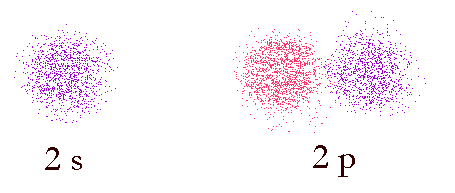
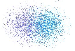
Image of probability domains of electrons in orbitals 2s and 2p. The color indicates the phase of the wave-function (the wave-like properties of the electron). In-phase functions add positively (constructive interference) and out of phase functions add negatively (destructive interference).
If we use one of these orbitals for one bond and the other for the other bond, we will obviously not have two identical bonds. We obviously need another model for the atomic orbitals in order to explain their participation in bonding. One thing many students forget when thinking of this process is that the orbitals them selves are not really entities and are not really the thing that matters. What matters is the overall energy of the system and its symmetry. An atom in free space is symmetrical (as much as its electrons will permit. The atomic orbitals s, p, d, f,… are merely the basis functions that we use to add up to the overall space occupied by the electrons. Note that any sub shell always adds up to be spherically symmetrical. We can easily choose a different set of basis functions (orbitals) to describe the space occupied by the electrons. Whatever basis set we use must exactly define the same space as our spdf model. We are free to divide up the space any way we want in order to more easily understand and calculate what we need.
Hybrid Orbitals (visualizations)
As an analogy, let’s consider a point in 2 dimensional cartesian space.
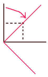
If the point is represent in the normal set of cartesian coordinates (basis set), we need an x value and a y value. On the other hand we can represent the same point using the alternate (rotated set) coordinate system (alternate basis set) In the rotated system, notice that one of the coordinates is zero (It still exists though.) and we can more easily ignore it in any calculations involving the point. We do the same with the space occupied by the atom’s electrons. Redefine the basis set we use so that we can simplify the mathematics.
What we need to do is use different (linear) combinations of the spdf domains to create new domains (orbitals).
We divide up the space (sphere) in such a way that each domain (orbital) of the sphere is involved in only one bond. This makes it much easier for any calculations we might have to do.
Let’s first consider what happens in the BeCl2 case:
First, we overlap the 2s and 2p in two different ways. (remember, we’re just creating new functions, not moving electrons)
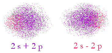
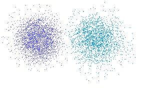
Here, we see that the two different ways of adding up the orbitals result in the phases interacting indifferent ways. In the 2s+2p case, the left-hand side will be smaller since the phases of the original s and p are opposite and vice versa for the 2s-2p case.
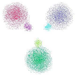
The two new orbitals we get will look like the following picture.
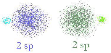
Two sp hybridized orbitals made from
an s and a p orbital. The two hybrid orbitals have axes that are 180° apart.
Now, we can see that the two different orbitals (coloured blue and green) still have properties that look like the p orbitals (two lobes, of different phase) and some properties like an s orbital (large bulbous, surrounding the nucleus (a bit). Most importantly, the two will sum up to make the same shaped space as has using the spdf model so these two orbitals will exactly describe the same space as the original s and p orbitals did. Now, we can look at using these to make molecular bonds.
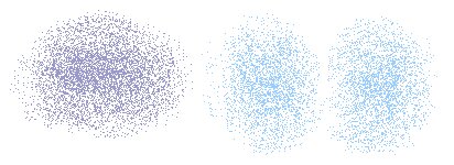
In the case of BF3, we have three fluorenes bonded to the central boron with what are experimentally observed to be identical bonds. Again, we cannot find a way of using the spdf model to easily describe the orbitals used for this so we will re-slice the sphere to make use of the space in a new way. First, we need only use three orbitals to create three bond so lets use s,p,p and leave one p orbital untouched on the atom.
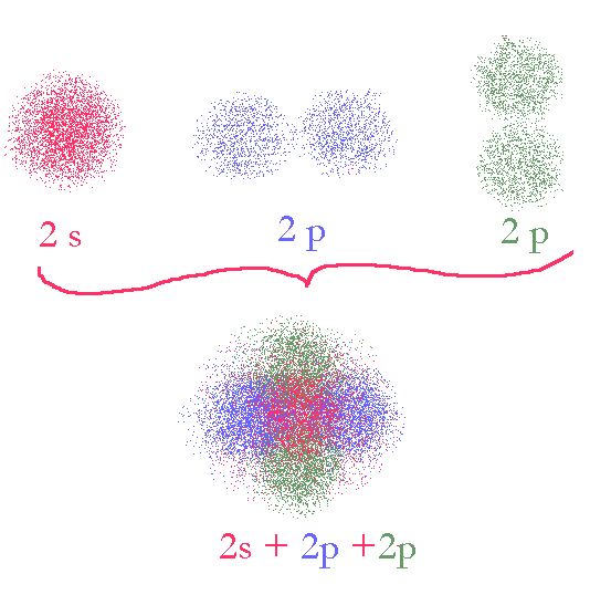
An s and two p orbitals add up their shapes to give a fat disk (note the color coding is used here to indicate different orbitals, not different phases). The three orbitals are 120° apart.
In the diagram here, we show the electron densities only resulting from each of three orbitals, s, p, p. colored differently If we add up the three sets of densities we get a picture of the space we need to divide up. It is a thick disk, sort of like a ball what is somewhat squashed in one direction. We now divide this up into three equal domains.
Three sp2 hybridized orbitals are made from an s and two p orbitals. Each hybrid has some p character and some s character.
and see that these three sp2 orbitals also add up to regenerate the original fat disk that the unhybridized spp combination added up to.
Here, we see the three orbital spaces added back together. Color coding helps remind us of the original sp2 hybridized orbitals.
The next set of hybrid orbitals is not so easy to show using these electron-cloud diagrams since the resulting set of hybrids will be evenly distributed in three dimensions rather than in just two. Hence, I will resort to stick diagrams to represent these orbitals.
In the molecule CH4 there are four equal electron domains on the carbon each involved in one bond with a hydrogen. How do we explain these using localized atomic orbitals.
First of all, recall that each sub shell will sum up to be a sphere. That means that if we add all the p orbitals with the s orbital for the n=2 level (or any n level), we still get a sphere. We divide the sphere into four equal parts and come up with domains that are 109.5° apart.
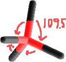
Here are the four sp3 hybrid orbitals after dividing up the space created by the s and the three p orbitals. The four new orbitals are all equal and have axes that are 109.5º apart.
More complicated hybridization can be found for atoms in the n > 3 shell. In these shells, there are d orbitals that can participate in the hybridizing. Thus, if an atom forms 5 bonds with 5 other atoms, it will need 5 atomic orbitals to do this. We take s, p, p, p, d of our n = 3 available orbitals and combine them. The resulting set of sp3d hybrids will have a trigonal bipyramidal arrangement exactly as describe in the VSEPR section. Finally, if there are six bond to six atoms, the hybridization will be sp3d2 (6 atomic orbitals needed) and the geometric arrangement of the electron domains will be octahedral (see VSEPR section).
In the Valence-bond approach, we assume that the molecules are made up by simply overlapping the atomic orbitals (hybridized if necessary) from the individual atoms. In this approach, the electrons from one atomic orbital AO don’t interact with those of other AOs. We get great three-dimensional pictures of what the molecules and bonds may look like but the information we can get from this approach is still not perfect. We’ll see MO theory later that can be used in parallel to obtain other information that this approach does a poor job at calculating.
We’ve seen various ways of visualizing atomic orbitals. It is important to remember that these orbitals are only models of what happens on an atom in the gaseous state (unattached to anything). How we deal with bonding these atoms together to form molecules is a whole different story again.
To form a bond between two atoms, we must overlap one atomic orbital (hybridized or not) from each of the two atoms that are bonded.
Two H atoms approach each other. Their Atomic Orbitals begin to overlap.

| The overlap space is shaped like a rugby ball. This is a σ1s bond. made by overlapping two 1s orbitals, one from each H atom. |
We see here the combination of two atomic s orbitals on Hydrogen atoms to form an H2 molecule. We can put the two electrons, one from each atom, into the new bond and we have a VB description of the bond in H2.
If we try to use VB theory to model the helium molecule, we run into problems. We see no place to put the four electrons as we only have one bond. Perhaps there is a lone pair, or something else. Experiment shows us that the He2 molecule does not exist in nature so that seems to correlate with the lack of places for all the electrons.
We will revisit this further. First, let’s look at a different type of bond. The σ bond we just looked at is a bond that has its major lobe on the axis joining the nuclei of the two atoms. A σ bond can be formed by the overlap of any type of orbitals contributed from the bonded atoms as long as the overlap occurs along the axis joining the two nuclei. This is in contrast to a π bond where the overlap is above and below (or on opposing sides) of the axis.
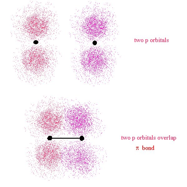
Here, the nuclei are represented by the two black dots. In the bond, we see that the overlap occurs off axis. It may be noticeable that the overlap is not as great as it could be if the lobes were overlapping end-to-end (σ bond)
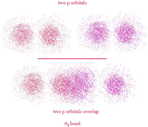
This time, the overlap occurs along the bond axis so this is a σ bond. We now see that the definition of σ and π bonds does not depend on the type of orbitals used in their creation. They refer to the location of the overlap region with respect to the bond axis.
single- and double-bonded atoms.
For some purposes, VB theory is convenient and easy to use, so we stick with it; hybridized orbitals coming together to form σ and the left-over atomic orbitals (p and d) form π bonds. This is most easily seen in organic molecules. The simplest of these is, of course, CH4 in which we’ve already seen the carbon atom to be sp3 hybridized and the carbon sp3 orbitals form σ bonds with the hydrogen s orbital. So far, we have looked only at molecules whose atoms are bonded together with single bonds.
What about a molecule with double bonds? Let’s look at the simplest of these; C2H4.
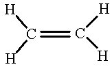
If we draw these orbitals, using solid lines to represent the shape of the orbitals rather than the electron-cloud images, we get something like the following.
First, we hybridize an s and two p orbitals on each carbon to form trigonal planer sp2 orbitals which we use in making σ bonds.
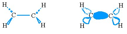
The σ bonds on the ethene molecule.
Now we look at the p orbital from each carbon that we didn’t yet touch and use it to form a π bond.
The π bonds on the ethene molecule
The complete picture looks like the following
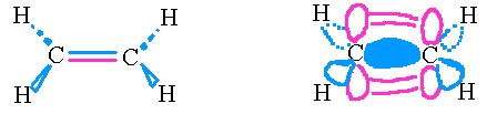
The σ and π bonds on the ethene molecule
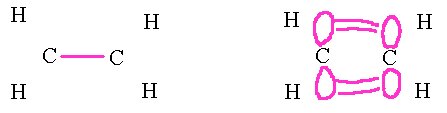
This scheme does a good job of helping us understand the properties of this molecule. We can see that the molecule is rigid and planar. It cannot rotate about the central C=C double bond because of the way the p orbitals overlap. We also see that the bond angle should be ca. the trigonal planar angle of 120°. the HCH angle is actually slightly smaller while the CCH angle is larger.
Triple bonds are even harder to draw. Consider the molecule ethyne C2H2. The carbons on this molecule are sp hybridized, leaving two p orbitals on each to form two π bonds. The final picture looks something like the following diagram.
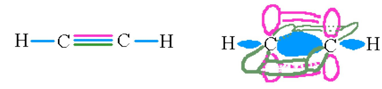
The σ and π and π bonds on the ethene molecule.
Again, we see this model does a reasonably good job of modeling the shape of the real molecule. Ethyne is linear and has a C≡C triple bond.
In both the cases previously, the bonds used are localized orbitals.
There are, however, many examples of organic and other molecules, which cannot be described simply using these localized orbitals and simple overlap. We have seen resonance as one method to try to overcome this deficiency. A better way it to allow that bonds and other orbitals in molecules (or complex ions) can be formed using more than just one orbital from each atom.
7.4:Molecular Orbital Theory
Molecular Orbital (MO) theory is a more accurate way to use calculations to predict molecular geometries and energies than VB theory. In MO theory, there is no hybridization and all orbitals on the molecule (now called molecular orbitals) can be made by combining any and all of the atomic orbitals from the individual atoms, unlike VB theory where bonds are made from only one orbital from each atom. This allows more flexibility in building up the mathematical picture of the molecule and results in a better match between theory and experimental data than we can get via VB theory.
Let’s revisit H2 and He2 using the MO approach. Using VB, we saw that we were unable to describe He2 and we concluded that the helium molecule must not exist. But that was somewhat unsatisfying. Using MO theory, we can build a model for He2 and we can use this model to explain why the molecule cannot exist in nature.
To form a bond between two atoms, we must combine atomic orbitals from the two atoms in such a way that the energy level of the combination (molecular orbital, MO) is lower than the original atomic orbital (AO). This is most easily visualized using the s orbitals of two hydrogen atoms as they approach each other. Consider, for a moment the following diagrams.

| Two H atoms approach each other. Their Atomic Orbitals begin to overlap. |
 Overall space is shaped like a rugby ball. This looks the same as we saw in VB theory but now, we need to account for the proper space. We started with two orbitals so we must finish with 2 orbitals. We now divide this space into two new (Molecular) orbitals
The best way to do this is such that the energy of the resulting molecule is lowest. In the case of hydrogen, there are two electrons to place in the new orbitals. If we define them such that one has a much lower energy than the other then we will see the stable molecule form when both electrons are situated in the low-energy orbital while the high-energy orbital is empty.
The division that best accomplishes this is one where the orbitals are added in phase (with normalization) and out of phase as is shown below.
in-phase out-of-phase
Molecular orbitals created by taking linear combinations of atomic orbitals (LCAO). On the left is the in-phase combination (addition) of the two atomic s orbitals (σ orbital; Bonding orbital) and on the right is the out-of-phase combination (subtraction) of the same two orbitals (σ* orbital; anti-bonding). These two add up to give the same space as the two original atomic orbitals but now each is a single ‘localized’ orbital spanning the whole molecule.
We see here the combination of two atomic s orbitals on Hydrogen atoms to form an H2 molecule. Just like in the atomic case, we always end up with the same number of orbitals that we started with. In this case, we’re jumping ahead of ourselves just a bit.
If we look at the energy of these two orbitals we come up with a correlation diagram like this
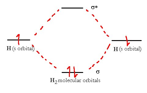
The Molecule H2 has an electron configuration (σ1s)2. It has an overall bond order of 1.
The two electrons from the hydrogen have a low-energy orbital and a high-energy orbital available to them. Provided they can lose energy (collision with the walls or a third atom or emission of light photon) the electrons will settle into the lower energy level and hence a net release of energy is observed. This released energy is called the bond energy.
The molecular electronic configuration can be named using molecular orbitals just as we saw in individual atoms. In this case, the only occupied orbital in the hydrogen atom is the s-orbital that was created from the 1s orbitals of the individual atoms. This molecular orbital (MO) is thus called a σ1s orbital. Thus, since both electrons are in this MO, we have a very simple molecular electron configuration (σ1s)2.
If we try the same thing using Helium. we can quickly see from the correlation diagram below why the helium does not form a He2 diatomic molecule.
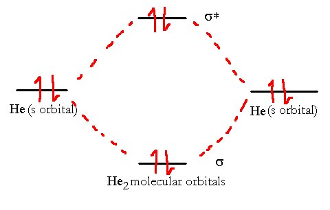
The He2 molecule will not remain stable since its overall bond order is zero. The MO electronic configuration is (σ1s)2(σ*1s)2, i.e., one bond and one antibond.
There are four electrons in the molecular orbitals which means that while two electrons can go to a lower energy level, the other two must go to the higher one. The total energy is unchanged. Hence, the two atoms don’t form a bond at all since there is no net release of energy.
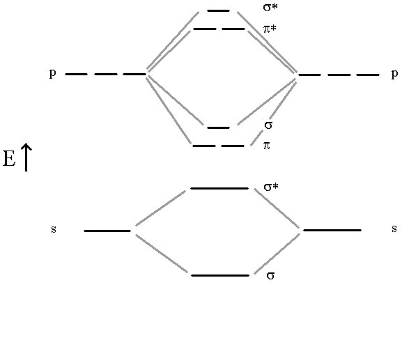
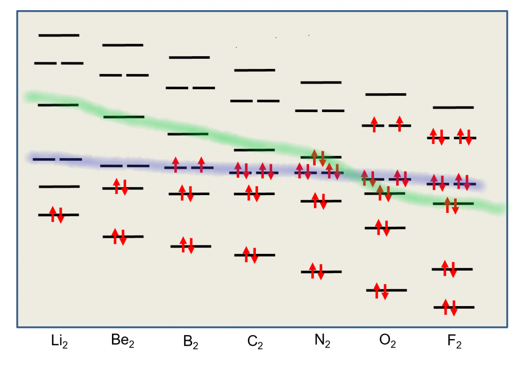
The previous model, for example is not useful at all in describing diatomic molecules like B2, C2, N2 and O2. For this, we need a more complete Molecular Orbital approach where all atomic orbitals can interact simultaneously to form molecular orbitals. In this approach, we don’t bother with the hybridization. All Atomic orbitals in the valence shell are involved in producing a molecular orbital scheme that mimics the experimentally observed properties. The four molecules mentioned above all use their n=2 valence shell to do the bonding. Let’s look at the correlation diagram that result when the 2s and 2p orbitals from two such atoms interact. It is important to note that the MO energy levels (σ2p) and (π2p) may not remain in this sequence for all atomic pairs. For example, the (π2p) levels are higher then the (σ2p) for O2 and F2. For our purposes, however, it will be sufficient to always use this one correlation diagram for any n=2 diatomic molecule, recognizing that it is not necessarily an exact representation of the energy levels for certain molecules.
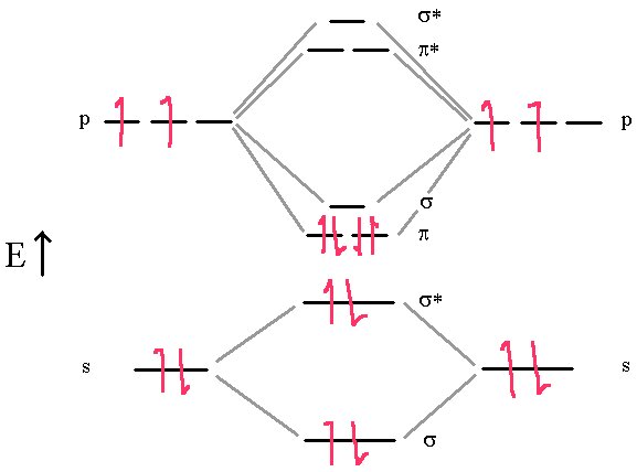
First, we’ll consider the Boron molecule. It has three electrons from each atom for a total of 6 electrons that we must place in the molecular orbitals. So the final scheme will look like the diagram below.
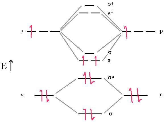
In this diagram, we can easily see that the MO electronic configuration is (σ2s)2(σ*2s)2(π2p)2 for an overall bond order of 1 ( (1 bond + 2 half bonds + 1 antibond)) but where the (π2p) orbitals contain unpaired electrons (Hund’s Rule) because they are degenerate (Identical energies).
This model predicts that the boron diatomic molecule is paramagnetic (two unpaired electrons). This is exactly what is observed experimentally. Note also that the bond order is essentially 1. The σ bond and σ* anti-bond cancel out, leaving the two π bonds each half occupied. How does this correlate with the Lewis dot structure?
![]()
The molecule of C2 is different. Experimentally, it is diamagnetic (no unpaired electrons) and has a bond order of 2.
In this diagram, we can easily see that the MO electronic configuration is (σ2s)2(σ*2s)2(π2p)4 for an overall bond order of 2 (3 bonds – 1 antibond).
We see that there are no σ bonds in carbon dimer. It is held together with π bonds only. This contradicts the other model where hybridization always predicts the first bond in a multiple bond is a σ bond.
Nitrogen molecules are triple bonded as we can see in the following diagram.
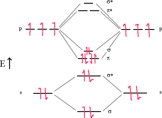
In this diagram, we can easily see that the MO electronic configuration is (σ2s)2(σ*2s)2(π2p)4(σ2p)2 for an overall bond order of 3 (4 bonds – 1 antibond).
We see that there is a (σ2p) bond and two (π2p) bonds holding the molecule together in this model. The (σ2s) and (σ*2s) cancel each other out and don’t contribute to the bonding.
Finally, Oxygen is paramagnetic with a bond-order of two. Lewis dot and VB theory doesn’t properly predict the paramagnetic properties. A good Lewis dot diagram of O2 shows a double bond with two lone pairs on each oxygen.
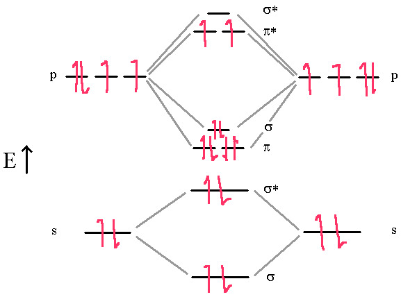
In this diagram, we can easily see that the MO electronic configuration is (σ2s)2(σ*2s)2(π2p)4(σ2p)2 (π*2p)2 for an overall bond order of 2 (4 bonds – 1 antibond – 2 half-filled antibonds). Again, the upper two electrons are unpaired in the π*2p degenerate orbitals. This molecule is paramagnetic because of Hund’s Rule.
Hund’s rule says we must put the last two electrons into the π* orbitals one at a time since they are degenerate orbitals. This gives us two unpaired electrons (Paramagnetic) and results in an overall bond order of 2.
We can use these same diagrams for diatomic molecules or ions for any combination of n=2 elements. for elements of n=3 or n=4, there is no guarantee that the sequence of the MOs will remain the same. It will always remain as pictured above for n=2 valence levels.
Let’s Try the NO molecule:
In this diagram, we can easily see that the MO electronic configuration is (σ2s)2(σ*2s)2(π2p)4(σ2p)2(π*2p)1 for an overall bond order of 2.5 (4 bonds – 1.5 antibonds). Here, the upper electron is unpaired in one of the two π*2p orbitals. They are no longer degenerate since one is empty. This molecule is paramagnetic, containing an odd number of electrons.
Note that there is an over-simplification in these diagrams. The atoms actually don’t always keep the same order of molecular orbitals from top to bottom. At oxygen, the order of the π2p and σ2p orbitals swap. any diatomic with oxygen or nitrogen has those two orbitals in reverse order in the MO energy diagram. But any answers you might need to answer (what is the bond order, what is the electron configuration, is it paramagnetic) will not change, so you can keep the same order for your simple MO diagrams.
7.5: Band Theory of solids
We’ve seen that metallic bonding can be thought of as an overlap of orbitals from neighbouring metal atoms, allowing the electrons to delocalize along the entire dimensions of the metal. We’ve also seen the concept that implies that the number of atomic orbitals must equal the number of molecular orbitals. We resolve these two concepts in the theory of bands. Bands are distributions of many molecular orbital energy levels, so closely spaced in energy that they seem to be continuous.
We will resolve the discussion of solids into three types, where bands are concerned:
|

7.5.1: Formation of bands
Let’s consider, a solid made up of a substance that involves only one type s of atomic orbital. For the moment, we’ll ignore the number of electrons the atom contributes. If we look at the chart below, we’ll see that at the number of such atoms with overlapping orbitals increases, so too does the number of molecular orbitals (and the MO energy levels)
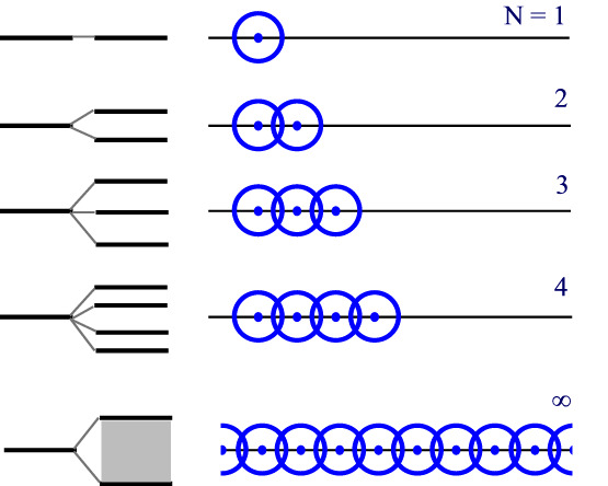
The set of energy for the N = ∞ case has N energy levels, so closely spaced that they appear continuous. This is a band of energy levels. This band is not uniformly spaced with the central energy levels occurring more closely packed than the highest and lowest levels in each band but that’s merely because of the way the orbitals overlap and is not an issue to this discussion.
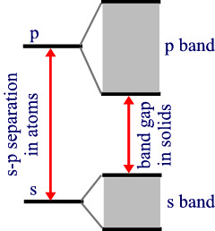
If the atoms involved have p orbitals available as well then multiple bands are available. J
ust as there were ene
rgy separations between the s and p orbitals on the atom that varied from atom to atom, there are band gaps that vary from solid to solid, depending on which atoms in the solid.
In each of these bands, we can consider the lowest energy levels to correspond to fully bonding molecular orbitals and the highest levels correspond to fully antibonding MOs.
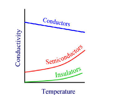
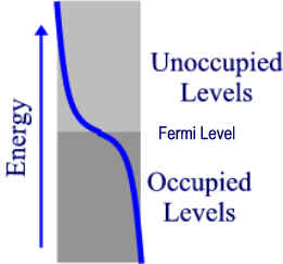 Now, lets look at the band occupancy. If the atoms we were considering (e.g. sodium) each contributes 1 electron then the band is exactly half filled. We need only consider the s band since it will made up of N atomic orbitals overlapped to give N energy levels with only N electrons. Thus the band occupancy can be represented by the diagram on the left. Actually, this diagram is only valid at absolute zero. At this temperature, the highest occupied level is called the Fermi level. As thermal energy is added to the solid, electrons become excited into some of the lower “Unoccupied” levels, giving a distribution of level occupancy called the Fermi-Dirac distribution (shown in blue for some T > 0 K). According to this equation, the higher the temperature above absolute zero, the higher the occupancy of the upper levels. However, the number of electrons in or near empty orbitals remains relatively constant throughout this process hence, no increase in conductivity occurs as a result of this process. Rather, as temp goes up, atoms vibrate more and collide with the moving electrons, creating “friction” or resistance, thus, conductivity decreases as temperature increases in conductors.
If the atoms involved in creating the gap each contribute 2 electrons then the s band would be exactly filled at T=0. Since, in most metals the s and p bands overlap slightly, there is no band gap and so mobility of electrons is still allowed.
7.5.2: Insulators and semiconductors
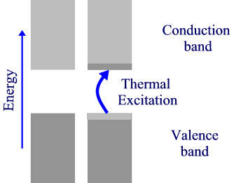
 If there is a non-zero band gap then we find a set of levels where the occupied levels and the unoccupied levels are separated. With increase in temperature above absolute zero, it becomes possible to excite some electrons from the highest of the occupied band (valence band) to the lowest of the unoccupied band (conduction band). Herein lies the distinction between insulators and semiconductors. in insulators, the band gap is large and only a negligible number of electrons are promoted at temperatures where the solid exists. Semiconductors, have smaller band gaps and significant promotion of electrons can occur from thermal excitation alone, causing conductivity to increase at T increases.
7.5.3: Doping
 If the solid semiconductor is doped with a low concentration of atoms that have different number of electrons then different band structures occur.
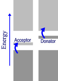
If (far left), the dopant atoms contain one less electron then there will be an extra unoccupied band slightly higher in energy than the valence band. This is called the acceptor band and can accept electrons from the valence band with lower thermal energies than the pure crystal bands can This is called a p-type semiconductor (P is for positive since the dopant atom will appear to have one fewer electrons, it will look to be “positive”).
If (left) the dopant atoms have extra electrons then an extra band is created that can donate electrons into the conduction band. This creates an n-type semiconductor. (N is for negative. the dopant atom has one more electron than the rest of the lattice and appears “negative” by comparison.
Combinations of n- and p-type semiconductors are used in the electronics industry to create diodes, transistors, etc. But That’s a whole new topic, which we won’t cover in this course.
7.6: Bond Dissociation Energies (D)
When bonds are formed energy is released. Electrons are in a more stable arrangement when in a bond (molecular orbital) than when they are unpaired (non-bonded) in atomic orbitals.
H2(g) 2H (g,atom) ΔH º = 436.0 kJ/mol
This is a bond-dissociation enthalpy or, bond enthalpy, or just bond energy.
We would write it as D(H-H) = 436.0 kJ/mol
We can use the bond-energies to calculate (approximate) enthalpies of formation for any compound.
take, for example H(g,atom). ΔfHº = 1/2 D(H-H).
1/2 H2(g) H(g,atom) ΔfHº = 218.0 kJ/mol
Consider the bonds in methane CH4. There are four C-H bonds.
| CH4(g) |
|
| ΔHº | = ΔfHº(C,g,atom) + 4 ΔfHº(H,g,atom) – ΔfHº(CH4,g) |
| = 716.7 kJ/mol + 4(218.0 kJ/mol) – (-74.5 kJ/mol) | |
| = 1663 kJ/mol | |
| D(C-H) | = ΔHº/4 = 1663 kJ/mol/4 = 415.8 kJ/mol |
Now, let’s consider the bonds in C2H6. There is one C-C bond and there are 6 C-H bonds.
| C2H6(g) |
|
| ΔHº | = 2 ΔfHº(C,g,atom) + 6 ΔfHº(H,g,atom) – ΔfHº(C2H6,g) |
| = 2(716.7 kJ/mol) + 6(218.0 kJ/mol) – (-84.7 kJ/mol) | |
| = 2826.1 kJ/mol | |
| We assume D(C-H) = 415.8 kJ/mol (same as for CH4). | |
| ΔHº | = D(C-C) + 6 D(C-H) |
| D(C-C) | = ΔHº – 6 D(C-H) = 2826.1 kJ/mol – 6 × 415.8 kJ/mol = 331.3 kJ/mol |
Ideally, we could continue like this and build up a complete list of all possible bond energies. From there, we could calculate the exact energies (enthalpies) of every chemical reaction without ever doing a single experiment. (in some ways, this is like the goal of many theoretical chemists; to be able to calculate the energies of the molecules and reactions in chemistry without need for actually doing the chemistry).
Unfortunately, the C-H bond in one compound is never quite the same as it is in any other compound. Therefore, this technique can at best give us rough approximations of certain reaction enthalpies. We wouldn’t want to push this idea very far as an analytical tool but it is very useful as a concept to understand reaction energies.
Bond energies from double and triple bonds
Consider the molecule C2H4 . There are four C-H bonds and one C=C bond.
We calculate the D(C=C) as follows:
| C2H4(g) |
|
| ΔHº | = 2 ΔfHº(C,g,atom) + 4 ΔfHº(H,g,atom) – ΔfHº(C2H4,g) |
| = 2(716.7 kJ/mol) + 6(218.0 kJ/mol) – 52.3 kJ/mol) | |
| = 2253.1 kJ/mol | |
| We assume D(C-H) = 415.8 kJ/mol (same as for CH4). | |
| ΔHº | = D(C=C) + 4 D(C-H) |
| D(C=C) | = ΔHº – 4 D(C-H) = 2253.1 kJ/mol – 4 × 415.8 kJ/mol = 589.9 kJ/mol |
Note that this is greater than D(C-C) but not twice as great, i.e., a double bond is not twice as strong as a single bond.
Once we have a table of bond energies, we can calculate ΔHº for a reaction by counting bonds broken and bonds formed and taking the algebraic sum of their energies. Remember bonds formed result in negative energy change for the system (exothermic) while bonds broken cause a positive energy change (endothermic). This equation would be written as
![]()
where i is the index of all bonds broken and j is the index of all bonds formed.
A simpler way of writing this is:
![]()
Alternatively, we assume all reactants are completely dissociates in to their atoms (all bonds are broken) and all products are formed from those elements.
![]()
This latter form might be confusing for some since normally, we think of products minus reactants and it is reversed here.
For example, estimate the enthalpy of combustion of ethane, given the bond energies below:
| bond type | Bond Energy / (kJ mol-1) |
| O-H | 464 |
| O=O | 498.4 |
| C=O | 804 |
| C-H | 414 |
| C-C | 347 |
The balanced chemical reaction is:
C2H6 + 7/2 O2 2 CO2 + 3 H2O
ΔHº = Σ D(broken) – Σ D(formed)
ΔHº = D(C-C) + 6 × D(C-H) + 3.5 × D(O=O) – 4 × D(C=O) – 6 × D(O-H)
ΔHº = 347 + 6 × 414 + 3.5 × 498.4 – 4 × 804 – 6 × 464
ΔHº = -1425 kJ/mol
Compare this value with that calculated using tabulated values of enthalpy of formation.
ΔHº = 2 × ΔHfº (CO2) + 3 × ΔHfº(H2O, g) – ΔHfº(C2H6) – 3.5 × ΔHfº(O2)
ΔHº = 2(-393.509) + 3(-241.818) – (-84.68) – 0
ΔHº = -1427.79 kJ/mol
7.7: Electronegativity
Experimental evidence leads us to recognize that not all covalent bonds involve the equal sharing of the electron pair in the bonds. Certain atoms attract the electrons in the bond pair more than other atoms. If a molecule contains two different types of atoms that are covalently bonded to each other, it is almost certain that the electron pair will not be equally shared. In the extreme, the bond is not a covalent bond but an ionic one.
7.7.1: Introduction
Linus Pauling ,(L. Pauling, The Nature of the Chemical Bond and the Structure of Molecules and Crystals, Cornell University Press: Ithaca, N.Y., 1948, pp. 58 – 75) used bond energies in his determination of a scale that could be used to measure the degree of unequal sharing or degree of ionic character in a bond. He used symbol  and
and  (Greek letter chi), to represent the electronegativities of atoms A and B, respectively.
There is no real way to calculate an atoms ability to pull electrons to itself in a covalent bond (a.k.a. electronegativity) without actually taking into account the other atom involved in the bond. We can calculate the difference in electronegativities using bond energies as the difference between the bond energies of the A-B molecule less the geometric average of the bond energies of the A-A and B-B molecules.
![\[\Delta = \Delta E_{AB} - \sqrt{\Delta E_{AA} \times \Delta E_{BB}}\]](https://ecampusontario.pressbooks.pub/app/uploads/quicklatex/quicklatex.com-af7e9b6b927abf4fd645a175cb45382d_l3.png "Rendered by QuickLaTeX.com")
The difference in the electronegativities can now easily be calculated using
![\[\chi_A - \chi_B = 0.102 \times \sqrt{\Delta}\]](https://ecampusontario.pressbooks.pub/app/uploads/quicklatex/quicklatex.com-461583e2c4cc73ea10873114d4503fa1_l3.png "Rendered by QuickLaTeX.com")
We rarely actually use these equations, relying mostly on tables of data compiled from large amounts of statistical data. Pauling originally set the value of the electronegativity for F to 4.00 and calculated other atoms’ electronegativities from there. Today, we use 3.98 for F, giving a scale with all atoms having electronegativities less than four and greater than zero.
Differences in electronegativities of two bonded atoms can be used as a predictor of the bond’s character. Differences greater than 2.0 are considered indicative of an ionic bond while differences less than about .4 indicate a pure covalent bond. Intermediate values for the electronegativity differences indicate a polar covalent bond where the electrons are not equally shared between the two atoms that are bonded.
Table of average Electronegativities calculated according to the method outlined above.
The Table of electronegativities as is most commonly found in textbooks. Numbers are scaled here to make F have exactly 4.0.
7.7.2: Dipole Moments
One last item we need to discuss while we’re on the topic of the three-dimensional structure of the molecules is their dipole moments. Dipole moments (μ) are caused by two opposite charges of magnitude δ in Coulombs separated by distance R in meters.
|μ|= δ · R.
Dipole moments are most often expressed in units of debye where 1 debye = 3.336×10⁻³⁰ coulomb meters.
Here, we can see that the larger the charge, the larger the dipole moment and the smaller the distance the smaller the moment. Thus molecules that have large charge separations can have large dipole moments. The absolute value sign around the symbol |m| is because this equation only represents the magnitude of the dipole moment. There is also a direction. We usually denote the direction as being from the positive to the negative charge. Thus, if two charges are separated by a distance as indicated in the diagram below, the dipole moment can be represented by a vector starting at the positively charged atom and going along the bond to the negatively charged one.
In theory, any bond that has charge separation of any amount will be polar although we may not be able to measure the polarity of some such bonds with very small charge separations. The only truly non polar bonds are those that are 100% covalent like the bond in a homonuclear diatomic molecule, e.g., H2, O2 or N2, etc.
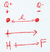 Here we can see an example of the HF molecule where two charges (both of magnitude d less than the magnitude of one electron charge, |d| < |e|) are separated by the bond length d of the molecule. Thus, we draw the dipole moment as a vector starting at the positive H (note the + sign) and pointing to the F atom. Unfortunately, the centre of the charge around each atom may not be exactly the centre of the nucleus so R is not necessarily the same as d.
We say that HF is polar since the molecule has a dipole moment.
In the case of more complicated molecules, we must add the vector dipole moments of each bond to get an overall dipole moment of the molecule. In the case of water, there are two bonds, each of which are polar.
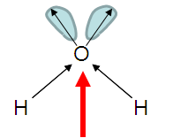 Here, we see that the two bond dipoles (red) lie along the H-O bond directions. These two add vectorially to produce a molecular dipole (red) that lies half-way between the two bonds. Additionally, the lone pairs increase the molecular dipole since they consist of significant negative concentration.
We call water a polar molecule because it has a molecular dipole.
In the case of BeCl2, there are two polar bonds but they are at 180° from each other and of the same magnitude. Thus, they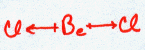 cancel each other out. There is no molecular dipole. The molecule is non-polar even though the bonds are polar.
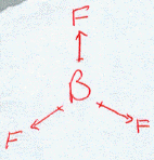 In this case, BF3, there are three bond dipoles, each at 120° from each other. These add vectorially in such a way as to cancel each other out. There is no molecular dipole and so the molecule is termed non-polar, even though the bonds themselves are polar.
The methane molecule has four polar bonds, as indicated in the picture. These are oriented at the tetrahedral angle of 109.5° from each other. again, these four bond dipoles cancel out so that the molecule becomes non-polar even though the bonds themselves are polar.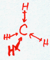
I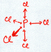 n Phosphorous pentachloride, it may not be quite so obvious but think of the equatorial (trigonal) ligands like that of the BF3. The dipole moments cancel out. The axial ligands are at 180° to each other and also cancel out. Thus, there is no molecular dipole even though the bonds are polar.
Similarly, the octahedral molecule SF6 would be non-polar despite the fact that all the bonds are polar.
In general, if any of these molecules’ symmetry is broken by reaction, they would become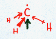 polar. For example, there is a species called the methyl radical. It is short-lived, highly reactive with a single electron where one hydrogen would have been. It is also polar as the picture shows. Similarly ammonia, NH3 with three hydrogens and a lone pair would be a polar molecule.
Thus, the polarity of a molecule depends not only on the polarity of the bonds in the molecule but also on its symmetry. Molecules with certain types of symmetry are not polar even if they have polar bonds.
Can we use these ideas to explain why ammonia (NH3) has a larger molecular dipole than NF3?
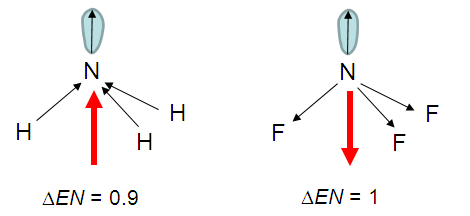
The polarity of the individual bonds would be similar (but in opposite directions) for NH3 as for NF3, however, in the case of the NH3, the lone pair’s negative concentration will augment the polarity contribution from the polar bonds while for the NF3, the lone pair’s dipole would subtract from the dipole contributed by the NF bonds.
Answers To Lewis Dot practice problems
CO3–2
 |
If we try joining all the atoms with single bonds, we get both O and C in non-normal valences. The O with only one bond looks like Li or F (which has three lone pairs that we don’t bother to show here yet). Li would make for a +6 formal charge so we’ll eliminate that one quickly as unreasonable. If the O is considered to be like F, it has a formal charge –1.The C has only a valence of 3 meaning it could look like B or like N. If we consider C to be isoelectronic with N (with a lone pair that is not drawn in yet) then the C would have a formal charge of –1 .
In this model the total of all the formal charges would add up to –4 but the actual species we’re trying to model has an overall charge of only –2, i.e., this model has too many electrons in it. |
|
 |
Here, we consider the possibility that the C looks like B and hence has a formal charge of +1.This gives us a valid Lewis dot structure since the sum of the formal charges does add up to the total charge. This means that once we put in our lone pairs, we will have the correct number of electrons. However, there is a better Lewis structure that we can draw, which has less formal charges. | |
 |
If we make a double bond the situation improves. Now, the C has a valence of 4 which is its normal valence and hence it has a formal charge of zero. One O (double bond) also has a normal valence (of 2) and a formal charge of zero. The two single-bonded oxygens still look like F and have a formal charge of –1 each. The formal charges add up to the overall charge on the species and we’ve lowered the total number of charges as much as we can. If we tried to create even more double bonds, we would create a hypervalent C which is not possible since C is an n = 2 atom and has no available d-orbitals.This is a good model which we’ll see later can be improved by using the concept of resonance. | |
 |
In this final diagram, we’ve added the lone pairs as follows:
|
|
| Now check electron sums |
    3O: 18
     C:  4
Charge:  2
   sum: 24 or 12 pairs.
|
If we count the electron pairs in our drawing we find 12 pairs exactly matching the number of valence electrons. |
O2
| Here, we’ve joined the O atoms with a single bond. They both look like F and would have a formal charge of –1 each for a total charge of –2. Obviously, wrong. | |
| Now, with a double bond, both O atoms are in their normal valence state with zero formal charge. This one looks good. | |
In this final diagram, we’ve added the lone pairs as follows:
|
|
| e– sums | 2O: 12 ==> 6 pairs, exactly as drawn in our Lewis dot structure. |
AlCl3
 |
Here, we’ve joined the atoms with single bonds. The Cl atoms are in their normal valence state and so are neutral. The Al is also in its normal valence state. This one was easy. | |
 |
Now, we’ve filled in the lone pairs on all the atoms according to their appearance in the table of normal and hypervalences. | |
| e– sums |
3Cl: 21 Al: 3 sum: 24 => 12 pairs |
we see 12 pairs of electrons in our Lewis dot structure exactly as predicted. |
IF3
| Here, we’ve joined the I and F atoms with single bonds. The F atoms are in their normal valence and have a formal charge of 0 each. The I is in its first hypervalent state and also has formal charge of 0. | ||
 |
In this final diagram, we’ve added the lone pairs as follows:
|
|
| e– sums |
3F: 21 I: 7 sum: 28 => 14 pairs |
We see 14 pairs drawn on the diagram |
XeF6
 |
Here, we’ve joined the F atoms to the Xe with a single bond. The F atoms are all in their normal valence state and would have a formal charge of 0. The Xe is in its third hypervalence state (check the table of normal and hypervalences) and also has a formal charge of 0. | |
 |
In this final diagram, we’ve added the lone pairs as follows:
|
|
| e– sums |
6F: 42 Xe: 8 sum: 50 => 25 pairs |
If we remember to count the the three lone pairs on each F which we didn’t draw in for simplicity sake, we find that we have indeed drawn 25 pairs of electrons. |
Numerical rules for making Lewis Structures.
Rules for creating Lewis Structures
So Far, I’ve created Lewis Structures for you pretty much ‘out of the air’. In some of the simple cases like H2O it is pretty obvious where all the electrons go. In the more complicated cases, multiple bonds, polyatomic ions, etc. It may not be quite so easy to decide the best structure.
Follow these few rules and you should have no trouble creating even quite complicated Lewis structures. I’ll enumerate the rules on the left hand side and prepare the structure of CO32– on the right-hand side as an example.
| Rule | Description | Example CO32– |
| 1 | Add up all the electrons in the valence shell, including those due to the charge. |
C ==> 4 3O ==> 18 2- ==> 2 total 24 |
| 2 | Draw a skeletal structure (single bonds only) paying attention as much as possible to the valence of the atoms. |  |
| 3 | Subtract from the total electron count, the number you used to make the single bonds |
24-6=18
or 9 pairs
|
| 4 | Add remaining electrons to the structure, starting with the most electronegative atoms first |  |
| 5 | Calculate the formal charge of the atoms (if they’re all zero, this is your last step) |
O: 6-6-1= -1 C: 4-0-3= +1 |
| 6 | Move electron pairs to create double bonds and thereby reducing formal charges as much as possible. Recheck the formal charges If there’s no further way you can reduce them you’re done. | 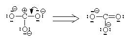 |
Note that over all of this, we must be aware of and keep the octet rule.
Let’s try another example. The common polyatomic anion, SO42–.
Count the electrons:
    S:  6
   4O: 24
Charge  2
total  32
Now draw the skeletal structure:

8 electrons used in the bonds. 32–8=24 electrons left to place (12 pairs). Calculate Formal Charge.
Now we reduce the formal charges on two of the oxygens and the sulfur by creating double bonds between the O and S using one lone pair from each of the two oxygens.
NOTE: This time we can violate the octet rule because sulfur’s valence electrons are in the n=3 shell which has 3-d orbitals where we can place electrons. Only elements in row 3,4,… of the periodic table can do this.
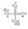
Note that there are five other possible combinations of oxygens on which I could have placed the double bonds and I still would have drawn an identical Lewis Structure. This leads us to the next topic of discussion. In reality, the oxygens on the sulfate ion are identical chemically. That means that any Lewis Structure which seems to make a distinction between the oxygens with and without double bonds is not completely correct.
