Chemical Equilibrium

Michael Mombourquette

12 Chemical Equilibrium

Michael Mombourquette

12.1: Introduction

Often (in our Stoichiometric calculations), we consider that reactions go to completion, i.e., that one or more of the reactants is completely used up.
This assumption is not always valid and in reality, is never 100% true.
Nothing is 100% in this world. There is no ‘pure’ substance, no ‘complete’ reaction, in a closed container but we can often make such an assumption with little or no additional uncertainty.
Any chemical system in a closed container will always reach a state of equilibrium. Sometimes that equilibrium state may be such that the container has almost no products or almost no reactants but it is still an equilibrium.
In an open system, some reactions can go to completion if it is arranged such that the product leaves the system as it is produced. For example, a liquid reaction mixture where one of the products is a gas. If the container is open and the gas is allowed to blow away then there can never be a reverse reaction as that particular component will be gone.

We will be exploring the more general cases where equilibrium is occurring. Equilibria can occur in solid, liquid or gas. We will start with gas phase equilibria as a simple reaction type but the general principles we explore here will still hold in other phases.

Consider the gas phase chemical system represent by the following chemical equation:

2 NO₂(g) ⇄ N₂O₄(g)

Reactants are reddish brown, products are colourless. Both temperature and pressure affect this equilibrium. Higher pressures (by compressing the container containing the reaction mixture) will favour the production of product (colourless) at the expense of the amount of reactant (coloured) hence, the equilibrium can be observed to change as the reaction vessel is compressed or expanded (as in a piston moving up and down in a glass cylinder.)

Definition: Equilibrium:: As it applies to a chemical reaction system: State of a reaction mixture at which the forward reaction rate is equal to the reverse reaction rate.

Note that there is no reference to the amounts of reactants necessary to achieve this state. This means that some equilibrium systems can have mostly reactants, others, mostly products and in rare cases, the same amount of reactants and products. It’s not the amount that is the deciding factor. Generally, the more the amount of reactant, or product, the faster will be the speed with which the forward, or reverse, reaction occurs. The relationship between the amount of material and the rate of reaction is given in the section on Kinetics, later in these notes. Suffice it to say, that most times, if the concentration of reactants goes up, the rate of conversion of these reactants to products goes up too.

Let’s look at a simple example:

The equilibrium between reactant A and product B: A ⇄ B

If there is initially, no B then there can be no reverse reaction. The Kinetic Molecular theory tells us that the rate of reaction depends somewhat on the collision frequency and that the collision frequency of molecules A with each other depends on how many molecules there are in the container. That seems to make sense. Therefore, as the amount of A is diminished from the initial situation (used up in the forward reaction) the forward rate will drop. Similarly, as the amount of B is increased due to the forward reaction, then the backward rate will increase from zero. eventually, a point will be reached where the forward and reverse rates are equal. At this point and until some stress is imposed on the system, reactants A are being produced and used up at equal rates and so are products B. Thus, although the reaction continues unabated, we see no overall changes to the amount of either A or B.

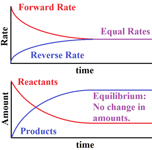
Fig. 1: shows measurable physical parameters for a system as it approaches equilibrium, starting from a conditions of only reactants and no products.

The Upper graph is a comparison of the magnitudes of the rates of forward and reverse reactions in the system as it approaches equilibrium. At the start of the reaction, there is only a forward reaction since there are no products yet to react. As time progresses, the magnitude of the forward rate diminishes and that of the reverse rate increases. Eventually (only after infinite time) the two magnitudes are equal and the chemical system has reached equilibrium. Note that I used magnitudes here. That is because by definition, the forward rate must be the negative of the reverse rate at equilibrium. For illustration purposes, I am only showing the magnitude of the rates here.

The Lower graph shows the amounts of Reactants and Products of the same system as it approaches equilibrium. Initially, there are only reactants but as time progresses, products are formed and reactants are used up. According to this graph, when equilibrium is reached the amounts of reactants and products no longer changes but are not necessarily equal to each other.

12.2: Equilibrium Constant

We need a way to describe the conditions under which a system will be at equilibrium. There are many combinations of different concentrations of products and reactants that will be possible at what are equilibrium conditions so it’s not a specific set of numbers that we’re looking for. Turns out it’s a ratio of concentrations of products divided by concentrations of reactants that we’re looking for. The particular ratio we’re interested in uses the coefficients of the balanced chemical equation as exponents.

Consider the reaction jA + kB ⇄lC + mD

The law of mass action (equil. const) gives us the following:

$K_c=\frac{[\mathrm{C}]^l[\mathrm{D}]^m}{[\mathrm{A}]^j[\mathrm{B}]^k}$

Note:
the square brackets [ ] indicate concentration in mol/L (M)
the subscript c on the K indicates this value derived using concentration units.

More generally, one can replace [A] by C_A where the capital C means Concentration in whatever units. Note that the units of K_c , assuming units of mol/L for the individual components, can be easily calculated to be

$\mathrm{(mol/L)}^{(l+m)-(j+k)}$

It can easily be determined that if l+m = j+k that there will be no units, in other words, the units will cancel.

If the reaction of interest is a gas phase one then we could replace the concentration C with pressure P. Thus we would now have defined a new type of equilibrium constant K_p as follows:

$K_p=\frac{P_C^l P_D^m}{P_A^j P_B^k}$

Note:
the equilibrium constant is calculated using pressures here. This value of the equilibrium constant may not be the same numeric value as the previously calculated equilibrium constant, except in the circumstances where the units exactly cancel out.
The subscript p on the K indicates this value derived using pressure units.

As we did above, we can calculate the units of K_p easily as

$\mathrm{(kPa)}^{(l+m)-(j+k)},$

assuming individual pressure units of kPa.
For a reaction where the special condition l+m = j+k exists. It matters not which units we use (pressure or Concentration) as the units will all cancel for a single phase reaction. For systems, where all units cancel, we see that K_c = K_p = K no matter what units we use.

Not all reaction systems are single phase systems. For example, reactions involving vapour pressure of some chemicals and liquid concentrations in the reaction mixture of others. These kinds of equilibrium constants would occur in dual phase reactions. For such an example, we cannot calculate either a K_c or a K_p since the units are not all pressure or all concentration. A more general form is the thermodynamic equilibrium constant, K. We need a better description of the ability of the chemicals to involve themselves in the reaction than concentration or pressure. This more general measure is called the activity of the chemical.

12.2.1: Activities

True Thermodynamic equilibrium constants are calculated using the activity (Test) of the components of the reaction. We will use a simplified definition, called the relative activity of a substance, which is related to some standard measure (concentration, pressure, etc) of that substance via

Relative activity (a) = measure/std measure.

For example, if concentrations are used, the units will be mol/L. The std concentration of an aqueous solution is 1M. Thus a substance A with concentration [A] (in M) would have relative activity a_A = [A] / 1 M (note in this case, the units were merely cancelled out by this process). Similarly, if gaseous substance A has partial pressure of p_A then the relative activity is a_A = p_A/p_Aº where p_Aº = 100 kPa. Thus, the thermodynamic equilibrium constant is written using activities as:

$K\;=\;\frac{a_C^\ell\,a_D^m}{a_A^j\,a_B^k}$

Since the individual activities are unitless, so too is the K constant. This is the kind of K constant we need in thermodynamic equations such as we will see in the thermodynamics section later. It is generally a good habit to start using this kind of K constant exclusively.

Example: Haber Process

Consider the process of converting hydrogen and nitrogen into ammonia. The simple looking gas phase reaction is useful to illustrate several points.

3 H₂ + N₂ ⇄ 2 NH₃

The thermodynamic equilibrium constant, i.e., calculated using activities, is defined as follows:

$K=\frac{a_{\mathrm{NH}_3}^2}{a_{\mathrm{H}_2}^3 \times a_{\mathrm{N}_2}}$

At room temperature the rate of this reaction is quite slow. It will seem to the casual observer that no reaction is occurring. At more elevated temperatures, the reactions speeds up and equilibrium is reached more quickly.
Example: At 127 ℃ the 3 following set of equilibrium concentrations were measured for a particular reaction mixture. What is the equilibrium constant K?

p_NH3 = 103 kPa
p_N2 = 2830 kPa
p_H2 = 10.3 kPa

The Thermodynamic equilibrium constant, defined above, uses activities. We need to convert the measured pressures into activities. We do this by dividing by the standard pressure of the gas. In units of kPa, the standard pressure is 100kPa. so we can thus write:

a_NH3 = 103 kPa/100 kPa = 1.03
a_N2 = 2830 kPa/100 kPa = 28.3
a_H2 = 10.3 kPa/100 kPa = .103

$K=\frac{a_{\mathrm{NH}_3}^2}{a_{\mathrm{H}_2}^3 \times a_{\mathrm{N}_2}}=\frac{1.03^2}{0.103^3\times 28.4}=34.3$
What if we had written the balanced chemical equation in terms of one mole of product (often done)?
We would have:

3/2 H₂ + 1/2 N₂ ⇄ NH₃

What is the equilibrium constant K’ now?

$K'=\frac{a_{\mathrm{NH}_3}}{a_{\mathrm{H}_2}^{3/2} \times a_{\mathrm{N}_2^{1/2}}}=\frac{1.03}{0.103^{3/2}\times 28.4^{1/2}}=5.86\equiv\sqrt{34.3}$

$K'=\sqrt{K}$

We could have also written the equation in reverse direction as:

NH₃ ⇄ 3/2 H₂ + 1/2 N₂

giving us

$K''=\frac{a_{\mathrm{H}_2}^{3/2} \times a_{\mathrm{N}_2^{1/2}}}{a_{\mathrm{NH}_3}}=\frac{0.103^{3/2}\times 28.4^{1/2}}{1.03}=\frac{1}{5.86} = 0.171$

$K''=\frac{1}{K'}$

Thus, we need to take care to associate the a particular equilibrium constant value with the correct associated equilibrium expression. The equilibrium constants of different forms of the same equation are, however, related, For example, if we double the coefficients of the balanced chemical equation, we double the exponents on the activities, i.e., we square the activities, and hence, we square the equilibrium constant value; if we halve the coefficients, then we halve the exponents (square root), etc. If we reverse the equation, we take the reciprocal of the K constant (multiply the exponents by -1).

12.3: Heterogeneous Equilibria

I mentioned in the last lecture that some equilibria can involve materials in different phases. We will discuss herein, how to handle some of these cases.

Consider the case of calcium carbonate decomposing to lime and carbon dioxide:

CaCO₃(s) ⇄ CaO(s) + CO₂(g)

The equilibrium constant expression is:

$K=\frac{a_{CaO}\times a_{CO_2}}{a_{CaCO_3}}$

However, the concentrations of the solids calcium carbonate and lime do not have an effect on the equilibrium. The activities of a pure solid (or liquid) are always close to one so they can be eliminated from the equation with no change in the outcome.

K = a_CO2.

Your own experience will be able to tell you this as well. Have you ever added sugar to a drink (say coolaid) to sweeten it up. If you are like most people, there was a time when sweet was the only taste you liked (childhood). In this case, you added as much sugar as you could before your mother or father took back the sugar dispenser and invariably, there was always some sugar left undissolved in the bottom of your glass. No matter how much sugar you added, only a certain amount of it actually dissolved. Although this is more of a physical process than a chemical process, the idea is the same. The amount of sugar in solution (concentration) was not affected by adding more solid sugar, its activity is simply 1, so there is no effect on the value of K.

Another example involving solids and gases follows:

NH₄HS (s) ⇄ NH₃ (g) + H₂S (g)

gives us

$K=\frac{a_{\mathrm{NH}_3}\times a_{\mathrm{H}_2\mathrm{S}}}{a_{\mathrm{NH}_4\mathrm{HS}}}$

We can simplify this expression because activity of pure NH₄HS solid is 1.

$K=a_{\mathrm{NH}_3}a_{\mathrm{H}_2\mathrm{S}}$

In the case of solution chemistry, where one of the phases is a liquid solution, we can approximate the same simplifications as long as the solutes are all dilute enough that we can assume the solvent’s activity is almost equal to 1. For example, in dilute aqueous solutions we make the approximation that the relative activity of the water is 1 but note that this is only a good approximation for dilute solutions.
Take for example, the acid base equilibrium of a weak acid with water, for example, Hydrogen Fluoride, HF.

HF(aq) + H₂O(l) ⇄F^–(aq) + H₃O⁺(aq)

The equilibrium constant expression for this equation is

$K=\frac{a_{\mathrm{F}^-}\times a_{\mathrm{H}_3\mathrm{O}^+}}{a_{\mathrm{HF}}}$

Note that we did not include the activity of the solvent, water, i.e., we assumed it’s activity is exactly 1. This is a good approximation as long as the concentrations of the solutes are all small. Then, the concentration of the water $C_{\mathrm{water}}$ will be almost identical to the standard concentration $(C^o_{\mathrm{water}}$ = $C_{\mathrm{pure water}})$ and so the relative activity $(C_{\mathrm{water}}/C^o_{\mathrm{water}})$ will be ~1.

12.4: Applications of the Equilibrium Constant

The equilibrium constants can be tabulated and used as necessary.

We can, for example, decide whether a particular reaction system will react nearly to completion (very large K) or almost not at all (very small K) or somewhere in between. The larger the value of K, the more the reaction will proceed to the right (more products). The smaller the value of K, the more the reaction will find equilibrium to the left (more reactants). We will look into this concept further in later lectures.

12.4.1: Reaction Quotient

Under conditions where the system is not at equilibrium or we are not sure if the system is at equilibrium, we cannot use measured activities to determine the equilibrium constant. We can still use the same formalism to calculate a parameter called the reaction quotient, Q. The reaction quotient is a parameter that tells us about the instantaneous conditions of the system, whether it is at equilibrium or not. Under the special conditions where the system is at equilibrium, then our new parameter, Q = K.

For a chemical system whether in equilibrium or not, we can calculate the value given by the law of mass action. Only if the system is at equilibrium will this value be the equilibrium constant. In general, we call this value the reaction quotient Q. Taking again the Haber equilibrium, we can write the reaction quotient for the system at any time.

3 H₂ + N₂ ⇄ 2 NH₃

$Q=\frac{a_{\mathrm{NH}_3}^2}{a_{\mathrm{H}_2}^3 \times a_{\mathrm{N}_2}}$

In this case, we are not necessarily using equilibrium concentrations and hence we calculated not the equilibrium constant K but the reaction quotient Q. We can now compare the two values as follows:

Q < K: This implies that the reaction is not at equilibrium and that the reaction must proceed to the right (make more products) to get to equilibrium.

Q = K: at this point the amount of products and reactants is just right to meet equilibrium conditions.

Q > K: implies that there are too many products. The reaction will proceed to the left to produce more reactant (and lower the among of product) until Q = K.

NOTE: if you are not using the relative activities to calculate Q and K, you must compare a Q_c with a K_c, a Q_p with a K_p etc.

Example

Consider the Haber equilibrium at 500℃. K = 3.5 × 10^-7. Predict which way the equilibrium will shift for each of the following cases.

	p_NH3	p_H2	p_N2
a.	4.16 kPa	8.3 kPa	403.5 kPa
b.	0.83 kPa	1470 kPa	6.20 kPa
c.	0.416 kPa	416 kPa	2.08 x 10⁴ kPa

Solution

a.

$Q=\frac{a_{\mathrm{NH}_3}^2}{a_{\mathrm{H}_2}^3 \times a_{\mathrm{N}_2}}$

$Q=\frac{(4.16/100)^2}{(8.3/100)^3 \times (403.5/100)}=0.75$

Since Q > K the reaction will proceed to the left until equilibrium.

b.

$Q=\frac{(0.83/100)^2}{(1470/100)^3 \times (6.20/100)}=3.50\times 10^{-7}$

Since Q = K the reaction is at equilibrium.

c.

$Q=\frac{(0.416/100)^2}{(416/100)^3 \times (2.08\times 10^4/100)}= 1.16 \times 10^{-9}$

Since Q < K the reaction will proceed to the right until equilibrium.^[1]

12.4.2: Calculating Equilibrium Pressures and Concentrations

Typically, we will be asked to find equilibrium concentrations (or pressures) given initial values. The basic technique for solving these problems is always the same. I will attempt to introduce you to the steps involved. Note, however that the exact execution of the steps may vary from problem to problem. In general this technique is called the ICE table technique, where the initials I,C,E stand for Initial, Change and Equilibrium, respectively. The point of this method is to determine the equilibrium values or expressions that we can then substitute into the equilibrium constant expression.

Determine the balanced chemical equation for the equilibrium in question. Be sure you used the correct formula (for example, does the K constant represent an equation where there is one mole of products etc…)
Set up the conditions (amounts of reactants and products present) not taking into account the equilibrium process itself, i.e., pretend you can artificially turn the equilibrium reaction off until you are ready.
Now turn on the equilibrium. amount x will react using up reactants and producing products. In some problems x is given, in others it is to be determined.
Do the calculations to find the unknown by substituting into the equilibrium constant expression for the balanced chemical reaction your wrote in step 1.

I will illustrate these steps by solving the following problem.

The reaction for the formation of gaseous hydrogen fluoride from hydrogen and fluorine has an equilibrium constant K of 1.15 × 10². 200.0 kPa of each cpd are added to a 1.5 L flask. Calculate the equilibrium partial pressures of all the species.

To do this, we use a technique called the ICE table calculation. In this technique, we tabulate the calculation process such that the columns correspond to each of the species in the balanced chemical reaction and the rows correspond to the steps in the calculations. These are: (I) Initial activities, (C) changes to these activities that are necessary to reach equilibrium, and finally, (E) the equilibrium activities.

	Balanced chemical equation
	H₂(g) + F₂(g)	2 HF (g)
Initial Relative activity (I).	2.000 2.000	2.000
No other preparation calculations are needed. We can let the reaction proceed to equilibrium. Let x be the overall amount of reaction, expressed as a relative activity. The individual changes can be determined from the stoichiometry as follows. Note that reactants are used up so the change is negative.
Change to reach equilibrium (C)	-x -x	+2x
Equilibrium Activities (I + C = E)	2.000-x 2.000-x	2.000+2x

Substitute the equilibrium values into the equilibrium constant expression for the balanced equation.

$K=1.15\times 10^2 = \frac{a^2_{\mathrm{HF}}}{a_{\mathrm{H}_2}\times a_{\mathrm{F}_2}}=\frac{(2.000+2x)^2}{(2.000-x)(2.000-x)}$

In this case, we can take the square root of both sides of the equation since this is easy to do. In other cases, you may need to do some other mathematical trick to make it work.

$\sqrt{1.15\times 10^2} = \frac{(2.000+2x)}{(2.000-x)}=10.7$

After some algebra, we get x = 1.528. Thus, the equilibrium relative activities can now be calculated:

a_H2	= a_F2	= 2.000 – 1.528	= 0.472
a_HF		= 2.000 + 2×1.528	= 5.056

Now, convert back to pressures from relative activities by multiplying by standard pressure.

p_H2	= p_F2	= 0.472 × 100 kPa	= 47.2 kPa
p_HF		= 5.056 × 100 kPa	= 505.6 kPa

This case was actually unusual in that the units cancelled out in the equilibrium constant expression and hence, K_c = K_p = K. and thus, we could have used partial pressures or concentrations directly in the equilibrium expression to arrive at the same numeric answer. Generally, you should use activities unless you see explicit units on the equilibrium constant.

We can do a check by recalculating K from these calculated pressures to see if the correct value is determined (it is).

This example was simple to solve only because we fortuitously chose initial amounts of reactants which made it possible to simplify the expression using a square root of the entire equation. Many times, these calculations require the use of the quadratic formula to obtain a solution.

Systems With Small K Constants

In some cases, we can take advantage of certain conditions to make some assumptions about the answer which will in turn make it easier to calculate the answer. We should always check any assumptions we make by calculation. I will illustrate the point with the following example

Gaseous NOCl decomposes incompletely to form NO and Cl₂ gases.

Given initially that 1.0 mol of NOCl is introduced into a 2.0 L container at 300 K with no NO or Cl₂ present, what are the equilibrium pressures?

$PV=nRT$

$P=\frac{nRT}{V}$

$P=\frac{1.0\times 8.314\; \mathrm{J/mol\; K}\times 300 \mathrm{K}}{2.0 \;\mathrm{L}}=1.2\times10^3\; \mathrm{kPa}$

Note that I pulled a fast one on you here. You should always convert all your units to SI to ensure that you get the correct numerical answer in the end. I didn’t convert L to m³. Why did it work?
The conversion of L to the SI units of m³ is 1000 L (a.k.a. kL) = 1 m³. That factor of a thousand is in the answer because I convert the unit Pa in the R value to kPa in the answer. This is a quick shortcut you can always do when using the ideal gas law. If you use volume in litres then you must use pressure in kiloPascals. Otherwise, use Pascals and cubic metres since they are the true SI units. This works because PV must be constant so using unit analysis, kL × Pa = L × kPa.

a_NOCl = 1.2×10³/100 = 12

The balanced chemical equation is:

	2 NOCl (g)	2 NO (g) +	Cl₂ (g)
Initial activity	12	0	0
Change	-2x	+2x	+x
Equilibrium Activity	12-2x	2x	x

and so we can substitute these equilibrium activities into the equilibrium expression:

$K=4.0\times10^{-11}=\frac{a_{NO}^2\times a_{Cl_2}}{a_{NOCl}^2}=\frac{(2x)^2\times x}{(12-2x)^2}$

Because the value K is at least two orders of magnitude smaller than the activity 12, we can try the following assumption.
We assume that the extent of reaction is small (since K is small) and hence x is small. We assume, in fact that x is so small that the denominator (12-2x) can be approximated by (12). (or another way of saying it is: assume that 2x << 12). Thus, we can now write

$K=4.0\times10^{-11}=\frac{(2x)^2\times x}{(12)^2}=\frac{4x^3}{(12)^2}$

$x^3=\frac{4.0\times10^{-11}\times (12)^2}{4}=1.44\times10^{-9}$

So

$x = 0.0011_{2924} \approx 0.00113$

.

Now check the validity of our assumption.

our assumption was	12 – 2×x ≈ 12
results show	12 – 2×0.00113 = 11_.998 ≈ 12 (subscript means not significant figure)

11.998 is .019% different from 12.^[2]

The arbitrary cut-off for these types of calculations is about 5% so this is a good assumption.

We can now calculate the equilibrium activities and from there, the partial pressures.

a_NOCl	= 12 – 2x ≈ 12 (rounded to two sig. figs)
a_NO	= 2x = 0.0023
a_Cl2	= x = 0.0011.

p_NOCl	= 12 × 100 = 1200 kPa
p_NO	= 0.0023 × 100 = 0.23 kPa
p_Cl2	= 0.0011 × 100 = 0.11 kPa

Again, we can check to see that our work is correct by substituting these into the equilibrium expression to see if we get the correct value for K (we do, within about 5%).

This technique of assuming that there was a small amount of reaction (small x) because of a small K value made the problem quite a bit easier to solve. This is valid most of the time if the K constant is at least two order of magnitudes smaller than the activities. You can see that in this case, we were borderline. Our answers were accurate to about 2 sig. figs. If we had need more precision on our numerical answers, we could not have made the assumption.

Systems With Large K Constants

Note: the final answer in the video for this question is wrong. The answer below, for the final pressure of methane is correct. Don’t let that distract you from the method used, which is correct in both the video and here in the text.

When the K constant is large, we can simplify the calculations by adding one extra step before using the Ice table. Since K is large, almost 100% of the reaction proceeds before reaching equilibrium. In this case, the amount of reaction (done the normal way) would be almost exactly the same as the amount of (the limiting) reagent and our calculations would be very difficult. If we first, pretend the reaction goes to completion and then allow it to reverse towards equilibrium, we get results that are easier to work with.

Consider the combustion reaction of 100 kPa of methane in excess oxygen (80kPa) to produce carbon monoxide and hydrogen gas.

CH₄(g) + 1/2 O₂(g) → CO (g) + 2 H₂(g) K = 1.4×10¹⁵

Lets do this first the normal way.

		CH₄(g) +	1/2 O₂ →	CO(s) +	2 H₂(g)
I	(pressures)	100kPa	80kPa	0	0
	(activities)	1.00	0.80	0	0

C		-x	-1/2x	+x	+2x

E		1.00-x	0.80-1/2x	x	2x

Thus, we get the following K expression after substituting these activities

$K=1.4\times 10^{+15}=\frac{x(2x)^2}{(1-x)(0.80-1/2x)^{1/2}}$

Thus, x = 0.9999999999999984.

Since only two sig. figs are valid, we would have to round up to 1.0 and from which we would have to assume that all CH₄ was used up (1 – x = 0). But we know that there is a measurable K constant so there must be a measurable amount of CH₄ at equilibrium.

Let’s try this again, first, we will do a limiting reagent calculation (in grey) to see which reagent is used up, how much of the other one is left over and how much of each product is produced. In this case, the limiting reagent calculation would show that all the methane is used up. We can quickly figure out the amount of oxygen used up and the products created using stoichiometry. Once the limiting reagent calculation is done, we can do the ICE table.

		CH₄(g) +	1/2 O₂ →	CO(s) +	2 H₂(g)
	(pressures)	100kPa	80kPa	0	0
	100% reaction Change	-100kPa	-(100/2) kPa	+100 kPa	+100×2 kPa
	(After the limiting reagent calc.)	0	30 kPa	100 kPa	200 kPa

I	(convert to activities)	0	0.30	1.00	2.00

C		+x	+1/2x	-x	-2x

E		x	0.30+1/2x	1.00-x	2.00-2x

$K=1.4\times10^{+15}=\frac{(1.00-x)(2.00-2x)^2}{(x)(0.30+1/2x)^{1/2}}$

We get $x = 5.2\times10^{-15}$ . The value of $x$ is at least 14 orders of magnitude smaller than the constants; obviously, our assumption about $x$ being small is valid.

Here, we assume that $x$ is small. In other words, we assume that

$1.00 - x = 1.00$

and

$2.00 - 2x = 2.00$

and

$0.30 + 1/2x = 0.30.$

Thus we are able to simplify the expression.

$K=1.4\times10^{+15}=\frac{1\times2^2}{x\times\sqrt{0.30}}$

Now, we multiply by 100 kPa to convert the equilibrium activity values into pressures so we can now report the amounts (pressures) of all the chemicals.

$\\p(CH_4) = 100 \; \textrm{kPa} \times 5.2\times10^{-15} = 5.2\times10^{-13}\; \textrm{kPa}.\\ p(O_2) = 30 \; \textrm{kPa}\\ p(CO) = 100 \; \textrm{kPa}\\ p(H_2) = 200 \; \textrm{kPa}.$

12.5: Le Châtelier’s Principle

A chemical system at equilibrium has many factors affecting the position of that equilibrium. The amount of each of the components, the temperature, the pressure (in gas phase reactions especially), presence of radiation, etc. We must be able to analyze these conditions and determine if one of them is changed what affect that will have on the position of the equilibrium.

The guiding light through all this is Le Châtelier’s Principle (LP). It states:

If a change (stress) is applied to a system at equilibrium the system will adjust to try to reduce the change.

Consider again the Haber process for the production of NH₃. Experience shows that the pressure and temperature both affect the equilibrium. Higher pressures give higher amounts of NH₃ and higher temperatures give lower amounts of NH₃ at equilibrium. looking at this data alone, one might think that high pressure, low temperature is a good set of conditions to produce high yields of ammonia. Unfortunately, at low temperatures, the rate of reaction is slower. A balance must be reached between the thermodynamic requirements for high yield and the kinetic requirements for achieving the results rapidly.

We will look at kinetics later. We will focus on the thermodynamic properties of the mixture as an example.

12.5.1: The Effect of a Change in Concentration

Consider the Haber process (3 H₂ + N₂ ⇄ 2 NH₃) at equilibrium with the following concentrations:

[N₂] = 0.399 M, [H₂] = 1.197 M, [NH₃] = 0.202 M.

What effect will the addition of N₂ to the system such that its concentration raises (instantaneously) by 1.000 M.

We can guess from LP that if addition of N₂ is the change then the equilibrium will shift to try to use up some of the extra N₂. The equilibrium will shift to the right. Calculation of Q will confirm this quantitatively.

Now, we can calculate the equilibrium constant from the equilibrium concentrations. In this case, we are merely doing a comparison of K with Q so we will just do the calculations using the concentration values rather than trying to convert to activities. It’s OK to do this as long as we are consistent. In other words, we are going to compare K_c with Q_c.

$K_c=\frac{[\mathrm{NH}_3]^2}{[\mathrm{H}_2]^3\times[\mathrm{N}_2]}=\frac{(0.202 M)^2}{(1.197 M)^3 (0.399 M)}=5.96\times10^{-2} M^{-2}$

We calculate the reaction quotient using the non-equilibrium conditions that result from the sudden change in concentration of the N₂ concentration to 1.399 M.

$Q_c=\frac{[\mathrm{NH}_3]^2}{[\mathrm{H}_2]^3\times[\mathrm{N}_2]}=\frac{(0.202 M)^2}{(1.197 M)^3 (1.399 M)}=1.70\times10^{-2} M^{-2}$

It’s obvious that Q_c < K_c and hence the equilibrium will shift to the right to produce more products (increasing Q until it is equal to K again). This is just what LP predicted qualitatively.

12.5.2: Effect of a Change in Pressure

There are three ways to affect a change in the pressure of a gaseous reaction mixture.

Add or remove a gaseous reactant or product.
Add an inert gas (not involved in the reaction).
Change the volume of the container.

We already considered the first option above.

The second will have no effect on a gas phase reaction (according to the assumptions made in deriving the ideal gas law). Since the partial pressures (or concentrations) of the individual gas components of the reaction do not change, an inert gas will not change the equilibrium.

If the volume of the container is changed, the individual pressures will change (and so will their concentrations). recall n_i/V = P_i/RT. If n_i is constant then when the volume V changes, the concentration (n_i/V) will change and so will P_i.

Qualitatively, we can use LP to predict the effect on an equilibrium if we re word the original definition slightly.

If a change in pressure is applied to a gaseous system at equilibrium the system will adjust to try to reduce the change in pressure.

Consider again the Haber process (3 H₂ + N₂ ⇄ 2 NH₃). We see that there are 4 moles of gas molecules in the reactant side and two moles of gas molecules in the product side (they’re all gases). Thus, if the equilibrium shifts to the right the pressure will drop and if it shifts to the left the pressure will rise.

Now consider a system at equilibrium (at some equilibrium pressure = sum of all partial pressures). If we squeeze the container so as to increase the pressure (of each partial pressure) we will change the equilibrium. LP predicts that the equilibrium will shift to the right to reduce the extra pressure. The new equilibrium will be reached where more products are present than before.

Exercise:

What will happen to the following reactions if the pressure is increased (by reducing the volume).

P₄(s) + 6 Cl₂ (g) ⇄ 4 PCl₃ (l) [answer1]
PCl₃(g) + Cl₂(g) ⇄ PCl₅(g) [answer2]
PCl₃(g) + 3 NH₃(g) ⇄ P(NH₂)₃(g) + 3 HCl(g) [answer3]

12.5.3: Effect of a Change in Temperature

The changes discussed so far have changed the equilibrium position but have not had effect on the equilibrium constant itself. Temperature changes will almost always cause a change in the equilibrium constant. To think about this using LP, we need to remember that all reactions involve the breaking of bonds (absorption of energy) and/or the formation of new ones (release of energy). It is exceedingly rare to find a chemical reaction where the energy absorbed is exactly equal to the energy released. In general we can assume that there is always some net change in energy involved in a chemical reaction. We need to consider this net change as a reactant or product to use LP.

Consider again the Haber process but this time note that energy is released during the process (exothermic).

3 H₂(g) + N₂(g) ⇄2 NH₃(g) + energy.

Now it’s easy to use LP to predict that if the temperature (kinetic energy) of the system is increased, the equilibrium will shift to the left to try to use up the excess energy. Since nothing else was changed, the new equilibrium position will have a different equilibrium constant than the old one. Since the new equilibrium has less products than the old one, the new K constant will be smaller than the old one (as T rises, K drops).

Temperature (K)	K
500	90
600	3
700	0.3
800	0.04

A reaction which consumes energy (endothermic) will have the opposite effect.

energy + CaCO₃(s) ⇄ CaO(s) + CO₂(g)

If the system initially at temperature T₁ with equilibrium constant (K₁) is warmed up to T₂ by adding energy, the reaction will shift to the right (to use up some of the extra energy), establishing a new equilibrium with a new K₂ > K₁.

We can represent this temperature dependence of K using the van’t Hoff equation. A rigorous derivation will be given for this equation later in this course.

$ln\left(\frac{K_2}{K_1}\right)=\frac{-\Delta H}{R}\left(\frac{1}{T_2}-\frac{1}{T_1}\right)$

Example:

The equilibrium constant for the Haber process

3/2 H₂ + 1/2 N₂ ⇄ NH₃

is 668 at 300 K and 6.04 at 400 K. What is the average enthalpy of reaction for the process in that temperature range?

$ln\left(\frac{668}{6.04}\right)=\frac{-\Delta H}{8.3145}\left(\frac{1}{300}-\frac{1}{400}\right)$

DH = -47 kJ/mol.

Looking up the value for DHº at 298.15 K, we find -46.11 kJ/mol, acceptably close to our estimated average value.

12.6: Real Gases

Up to this point, we’ve always been using the ideal gas approximations when discussing equilibrium constants, etc, where gases were involved. In reality, there are few gases which behave in an ideal way except at pressures which are relatively low and temperatures that are not very low. Higher pressures result in properties of gases which deviate from ideal behavior quite appreciably.

Consider again the Haber process (at 723 K).

3 H₂(g) + N₂(g) ⇄2 NH₃(g)

The K_p value we calculate using observed partial pressures would be

$K_p^{obs}=\frac{(p_{\mathrm{NH}_3}^{obs})^2}{(p_{\mathrm{H}_2}^{obs})^3 \times(p_{\mathrm{N}_2}^{obs})}$

Since the observed pressure deviates from ideal pressure noticeably at high pressure, this calculated value will be in some error and the error will increase as pressure increases. See the table below for a set of pressures and observed equilibrium constants to illustrate this point.

Total Pressure (atm)	K_p^obs (atm^-2)
10	4.4×10^-5
50	4.6×10^-5
100	5.2×10^-5
300	7.7×10^-5
600	1.7×10^-4
1000	5.3×10^-4

We can correct for this error using a more complete definition for activities. This will not be discussed further here in first-year Chemistry. You will see discussions on this topic if you take upper year Physical Chemistry courses later in your career.

Table: Some important gas phase reactions

$\begin{array}{lllll} \hline \textrm{Reaction} & K(25^\circ C)& \DeltaH^\circ(25^\circ C)& \Delta n_g& \textrm{Typical}\\ & & \textrm{kJ/mol} & \textrm{moles} & \textrm{conditions}\\ \hline \textrm{Sulfur trioxide}\\ \mathrm{SO_2 + 1/2 O_2 \rightleftarrows SO_3}&2.7\times10^{12}& -98.8& -0.5 & 500^\circ C\\ \mathrm{Ammonia}\\ \mathrm{N_2 + 3 H_2 \rightleftarrows 2 NH_3}& 7.6\times10^2& -46.1& -2& 450^\circ, 100\textrm{MPa}\\ \textrm{Synthesis gas} \\ \;\;\textrm{Steam Reforming}\\ \;\;\mathrm{CH_4 + H_2O \rightleftarrows CO + 3 H_2}& 1.3\times10^{-25}& +206.1 & +2 & 900^\circ C\\ \;\;\textrm{Shift Conversion}\\ \;\;\mathrm{CO + H_2O \rightleftarrows CO_2 + H_2} & 1.0\times10^5 & -41.2 & 0 & 300^\circ C\\ \;\;\textrm{Partial oxidation of methane}\\ \;\;\mathrm{CH_4 + 1/2 O_2 \rightleftarrows CO + H_2} & 1.4\times10^{15} & -35.7 & +1.5 & 1400^\circ C, 2 \textrm{MPa}\\ \;\;\textrm{Water gas}\\ \;\;\mathrm{C(s) + H_2O \rightleftarrows CO + H_2} & 9.8\times10^{-17} & +131.3 & +1 & 1000^\circ\\ \;\;\textrm{Fisher Tropsch}\\ \;\;\mathrm{CO + 2H_2 \rightleftarrows CH_4 + H_2O} & 7.7\times10^{24} & -206.1 & -2\\ \textrm{Methanol}\\ \mathrm{CO + 2H_2 \rightleftarrows CH_3OH} & 2.2\times10^4 & -90.1 & -2 & 300^\circ, \textrm{30 MPa}\\ \textrm{Ethylene}\\ \mathrm{H_3C-CH_3 \rightleftarrows H_2C=CH_2 + H_2} & 2.1\times10^{-18} & +136.9 & +1 & 750-900^\circ \end{array}$

Note that there is a typo in the answer to this in the video. It has the answer to part C as $1.16\times 10^{-13}$ , which is wrong but the rest of the conclusions are right. this error stems from a missing decimal point in the nitrogen pressure. ↵
The percent difference between a known value A and a calculated value B is:
% dif $= \frac{|A-B|}{A}\times 100 \%$

In our example, A = $12$ and B = $12-2\times.00113}$ . So their difference is $2\times 0.00113$ and hence the percent difference is

% dif $= \frac{|2\times0.00113|}{12}\times 100\% = 0.019\%$ ↵