Chapter 2.2: Graphing Linear Equations

Mike LePine

Chapter 2.2: Graphing Linear Equations

There are two common procedures that are used to draw the line represented by a linear equation. The first one is called the slope-intercept method and involves using the slope and intercept given in the equation.

If the equation is given in the form $y = mx + b$ , then $m$ gives the rise over run value and the value $b$ gives the point where the line crosses the $y$ -axis, also known as the $y$ -intercept.

Example 1

Given the following equations, identify the slope and the $y$ -intercept.

$\begin{array}{lll} y = 2x - 3\hspace{0.14in} & \text{Slope }(m)=2\hspace{0.1in}&y\text{-intercept } (b)=-3 \end{array}$
$\begin{array}{lll} y = \dfrac{1}{2}x - 1\hspace{0.08in} & \text{Slope }(m)=\dfrac{1}{2}\hspace{0.1in}&y\text{-intercept } (b)=-1 \end{array}$
$\begin{array}{lll} y = -3x + 4 & \text{Slope }(m)=-3 &y\text{-intercept } (b)=4 \end{array}$
$\begin{array}{lll} y = \dfrac{2}{3}x\hspace{0.34in} & \text{Slope }(m)=\dfrac{2}{3}\hspace{0.1in} &y\text{-intercept } (b)=0 \end{array}$

When graphing a linear equation using the slope-intercept method, start by using the value given for the $y$ -intercept. After this point is marked, then identify other points using the slope.

This is shown in the following example.

Example 2

Graph the equation $y = 2x - 3$ .

First, place a dot on the $y$ -intercept, $y = -3$ , which is placed on the coordinate $(0, -3).$

Graph with intercept at (0,-3)

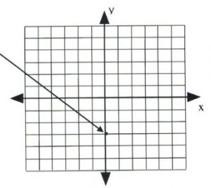
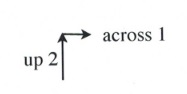
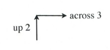
Now, place the next dot using the slope of 2.

A slope of 2 means that the line rises 2 for every 1 across.

Simply, $m = 2$ is the same as $m = \dfrac{2}{1}$ , where $\Delta y = 2$ and $\Delta x = 1$ .

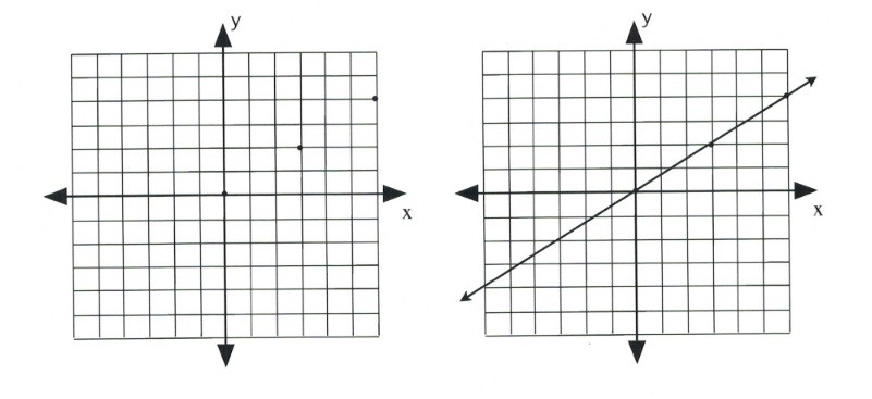
Placing these points on the graph becomes a simple counting exercise, which is done as follows:

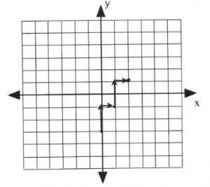
For m = 2, go up 2 and forward 1 from each point.

From each point, go up 2 and forward 1 to find the next point.

Once several dots have been drawn, draw a line through them, like so:

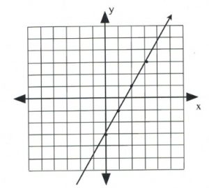
Line with slope of 2. Passes through (−3, 0), (1, −1), (2, 1), and (3, 3).

Note that dots can also be drawn in the reverse of what has been drawn here.

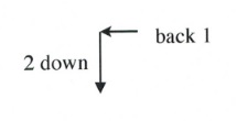
Slope is 2 when rise over run is $\dfrac{2}{1}$ or $\dfrac{-2}{-1}$ , which would be drawn as follows:

For m = 2, go down 2 and back 1 from each point.

Example 3

Graph the equation $y = \dfrac{2}{3}x$ .

First, place a dot on the $y$ -intercept, $(0, 0)$ .

Now, place the dots according to the slope, $\dfrac{2}{3}$ .

When m = 2 over 3, go up 2 and forward 3 to get the next point.

This will generate the following set of dots on the graph. All that remains is to draw a line through the dots.

Line with slope 2 over 3. Passes through (−3, −2), (0, 0), (3, 2), and (6, 4).

The second method of drawing lines represented by linear equations and functions is to identify the two intercepts of the linear equation. Specifically, find $x$ when $y = 0$ and find $y$ when $x = 0$ .

Example 4

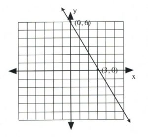
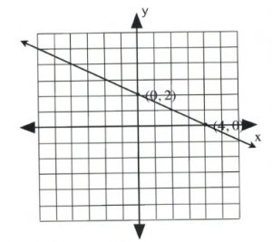
Graph the equation $2x + y = 6$ .

To find the first coordinate, choose $x = 0$ .

This yields:

$\begin{array}{lllll} 2(0)&+&y&=&6 \\ &&y&=&6 \end{array}$

Coordinate is $(0, 6)$ .

Now choose $y = 0$ .

This yields:

$\begin{array}{llrll} 2x&+&0&=&6 \\ &&2x&=&6 \\ &&x&=&\frac{6}{2} \text{ or } 3 \end{array}$

Coordinate is $(3, 0)$ .

Draw these coordinates on the graph and draw a line through them.

Line with slope of 2. Passes through (0, 6) and (3, 0).

Example 5

Graph the equation $x + 2y = 4$ .

To find the first coordinate, choose $x = 0$ .

This yields:

$\begin{array}{llrll} (0)&+&2y&=&4 \\ &&y&=&\frac{4}{2} \text{ or } 2 \end{array}$

Coordinate is $(0, 2)$ .

Now choose $y = 0$ .

This yields:

$\begin{array}{llrll} x&+&2(0)&=&4 \\ &&x&=&4 \end{array}$

Coordinate is $(4, 0)$ .

Draw these coordinates on the graph and draw a line through them.

Line with negative slope. Passes through (0, 2) and (4, 0).

Example 6

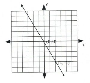
Graph the equation $2x + y = 0$ .

To find the first coordinate, choose $x = 0$ .

This yields:

$\begin{array}{llrll} 2(0)&+&y&=&0 \\ &&y&=&0 \end{array}$

Coordinate is $(0, 0)$ .

Since the intercept is $(0, 0)$ , finding the other intercept yields the same coordinate. In this case, choose any value of convenience.

Choose $x = 2$ .

This yields:

$\begin{array}{rlrlr} 2(2)&+&y&=&0 \\ 4&+&y&=&0 \\ -4&&&&-4 \\ \midrule &&y&=&-4 \end{array}$

Coordinate is $(2, -4)$ .

Draw these coordinates on the graph and draw a line through them.

Line with negative slope. Passes through (0, 0) and (2, −4).

Questions

For questions 1 to 10, sketch each linear equation using the slope-intercept method.

$y = -\dfrac{1}{4}x - 3$
$y = \dfrac{3}{2}x - 1$
$y = -\dfrac{5}{4}x - 4$
$y = -\dfrac{3}{5}x + 1$
$y = -\dfrac{4}{3}x + 2$
$y = \dfrac{5}{3}x + 4$
$y = \dfrac{3}{2}x - 5$
$y = -\dfrac{2}{3}x - 2$
$y = -\dfrac{4}{5}x - 3$
$y = \dfrac{1}{2}x$

For questions 11 to 20, sketch each linear equation using the $x\text{-}$ and $y$ -intercepts.

$x + 4y = -4$
$2x - y = 2$
$2x + y = 4$
$3x + 4y = 12$
$2x - y = 2$
$4x + 3y = -12$
$x + y = -5$
$3x + 2y = 6$
$x - y = -2$
$4x - y = -4$

For questions 21 to 28, sketch each linear equation using any method.

$y = -\dfrac{1}{2}x + 3$
$y = 2x - 1$
$y = -\dfrac{5}{4}x$
$y = -3x + 2$
$y = -\dfrac{3}{2}x + 1$
$y = \dfrac{1}{3}x - 3$
$y = \dfrac{3}{2}x + 2$
$y = 2x - 2$

For questions 29 to 40, reduce and sketch each linear equation using any method.

$y + 3 = -\dfrac{4}{5}x + 3$
$y - 4 = \dfrac{1}{2}x$
$x + 5y = -3 + 2y$
$3x - y = 4 + x - 2y$
$4x + 3y = 5 (x + y)$
$3x + 4y = 12 - 2y$
$2x - y = 2 - y \text{ (tricky)}$
$7x + 3y = 2(2x + 2y) + 6$
$x + y = -2x + 3$
$3x + 4y = 3y + 6$
$2(x + y) = -3(x + y) + 5$
$9x - y = 4x + 5$

Answers to odd questions.

1. $m=2$

3. $m=4$

5. $\begin{array}{rrrrlrrr} \\ \\ \\ \\ x&-&y&=&4&&& \\ -x&&&&-x&&& \\ \midrule &&(-y&=&-x&+&4)&(-1) \\ &&y&=&x&-&4& \\ &&m&=&1&&& \end{array}$

7. $\begin{array}{rrlrrr} \\ \\ \\ \\ \\ y&=&\dfrac{1}{3}x&&& \\ \\ \therefore m&=&\dfrac{1}{3} &&& \\ m_{\perp} &=&-1&\div &\dfrac{1}{3}&\text{or} \\ m_{\perp}&=&-3 &&& \end{array}$

9. $\begin{array}{lrlrrrr} \\ \\ \\ \\ m&=&-\dfrac{1}{3} &&&& \\ m_{\perp} &=&-1&\div &-\dfrac{1}{3}&&\\ \\ m_{\perp}&=&-1 &\cdot &-\dfrac{3}{1}&=& 3 \end{array}$

11. $\begin{array}{rrrrlrr} \\ \\ \\ \\ \\ \\ \\ \\ x&-&3y&=&-6& \\ -x&&&&-x&& \\ \midrule &&\dfrac{-3y}{-3}&=&\dfrac{-x}{-3}&-&\dfrac{6}{-3} \\ \\ &&y&=&\dfrac{1}{3}x&+&2 \\ &&m_{\perp}&=&-1&\div &\dfrac{1}{3} \\ &&m_{\perp}&=&-3&& \end{array}$

13. $\begin{array}{rrrrlrr} \\ \\ \\ \\ \\ \\ \\ \\ \\ \\ m&=&\dfrac{2}{5}&&&& \\ \\ y&-&y_1&=&m(x&-&x_1) \\ y&-&4&=&\dfrac{2}{5}(x&-&1) \\ \\ y&-&4&=&\dfrac{2}{5}x&-&\dfrac{2}{5} \\ \\ &+&4&&&+&4 \\ \midrule &&y&=&\dfrac{2}{5}x&+&\dfrac{18}{5} \end{array}$

15. $\begin{array}{rrrrlrr} \\ \\ \\ \\ \\ \\ \\ \\ \\ \\ m&=&\dfrac{1}{2}&&&& \\ \\ y&-&y_1&=&m(x&-&x_1) \\ y&-&4&=&\dfrac{1}{2}(x&-&3) \\ \\ y&-&4&=&\dfrac{1}{2}x&-&\dfrac{3}{2} \\ \\ &+&4&&&+&4 \\ \midrule &&y&=&\dfrac{1}{2}x&+&\dfrac{5}{2} \end{array}$

17. $\begin{array}{rrrrlrr} \\ \\ \\ \\ \\ \\ \\ \\ \\ \\ m&=&-\dfrac{3}{5}&&&& \\ \\ y&-&y_1&=&m(x&-&x_1) \\ y&-&3&=&-\dfrac{3}{5}(x&-&2) \\ \\ y&-&3&=&-\dfrac{3}{5}x&+&\dfrac{6}{5} \\ \\ &+&3&&&+&3 \\ \midrule &&y&=&-\dfrac{3}{5}x&+&\dfrac{21}{5} \end{array}$

19. $\begin{array}{rrrrrrrrr} \\ \\ \\ \\ \\ \\ \\ \\ \\ \\ -x&+&y&=&1&&&& \\ +x&&&&+x&&&& \\ \midrule &&y&=&x&+&1&& \\ &&\therefore m&=&1&&&& \\ \\ y&-&y_1&=&m(x&-&x_1)&& \\ y&-&-5&=&1(x&-&1)&& \\ y&+&5&=&x&-&1&& \\ -y&-&5&&-y&-&5&& \\ \midrule &&0&=&x&-&y&-&6 \end{array}$

21. $\begin{array}{rrrrrrrrrr} \\ \\ \\ \\ \\ \\ \\ \\ \\ \\ \\ 5x&+&y&=&-3&&&&& \\ -5x&&&&-5x&&&&& \\ \midrule &&y&=&-5x&-&3&&& \\ &&\therefore m&=&-5&&&&& \\ \\ y&-&y_1&=&m(x&-&x_1)&&& \\ y&-&2&=&-5(x&-&5)&&& \\ y&-&2&=&-5x&+&25&&& \\ -y&+&2&&-y&+&2&&& \\ \midrule &&(0&=&-5x&-&y&+&27)&(-1) \\ &&0&=&5x&+&y&-&27& \end{array}$

23. $\begin{array}{rrrrrrrrr} \\ \\ \\ \\ \\ \\ \\ \\ \\ \\ -4x&+&y&=&0&&&& \\ +4x&&&&+4x&&&& \\ \midrule &&y&=&4x&&&& \\ &&\therefore m&=&4&&&& \\ \\ y&-&y_1&=&m(x&-&x_1)&& \\ y&-&2&=&4(x&-&4)&& \\ y&-&2&=&4x&-&16&& \\ -y&+&2&&-y&+&2&& \\ \midrule &&0&=&4x&-&y&-&14 \end{array}$

25. $y=-3$

27. $x=-3$

29. $y=-1$

31. $x=-2$

33. $y=3$

35. $x=5$

License

Icon for the Creative Commons Attribution-NonCommercial-ShareAlike 4.0 International License

Questions

License

Share This Book