5.7 Introduction to Graphing Polynomials
Learning Objectives
By the end of this section, you will be able to:
- Graph a basic polynomial function of the form [latex]f(x)=ax^2+k[/latex].
- Graph a basic polynomial function of the form [latex]f(x)=ax^3+k[/latex].
In this section, we will focus on graphing simple polynomial functions by identifying some important characteristics and creating a table of values. Polynomial functions can be represented graphically in the rectangular coordinate system, and these graphical representations can allow us to learn about the function visually and better understand the relationship between the variables. Polynomial functions can undergo many transformations to their form, but in this section, we will focus on vertical reflections and translations only.
Please note that the figures created for this section were created using the desmos graphing calculator. Feel free to use this calculator in your studies to better understand the graph of functions.
Graphs of Quadratic Equations
Let’s examine the general shape of a graph of a general quadratic function [latex]f(x)=ax^2[/latex]. The graph of a quadratic equation is called a parabola.
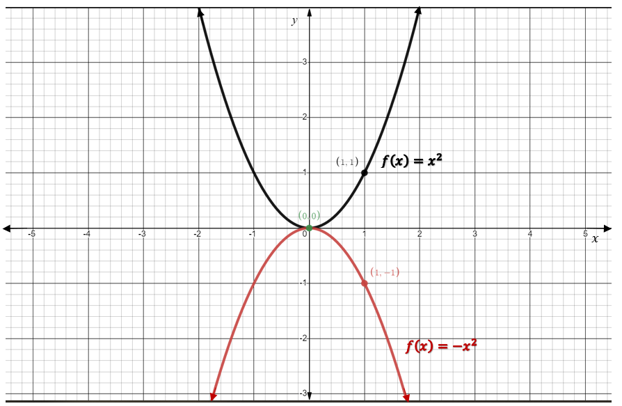
In the figure below (Figure 5.7.1), we see the graphs of the functions [latex]f(x)=x^2[/latex] and [latex]f(x)=-x^2[/latex]. Notice that the only difference between these two equations is the sign in front of the [latex]x^2[/latex]. This shows us that the sign of the leading coefficient, [latex]a[/latex], determines the direction of opening of a parabola. If the leading coefficient of a quadratic function is positive, [latex]a>0[/latex], the parabola will open upwards, whereas if the leading coefficient of a quadratic function is negative, [latex]a<0[/latex], the parabola will open downwards.
Quadratic Equations Direction of Opening
For a function of the form [latex]f(x)=ax^2[/latex],
if [latex]a>0[/latex], the parabola opens upwards.
if [latex]a<0[/latex], the parabola opens downwards.
Another important characteristic of a parabola is its vertex. Here, we see that the vertex is the origin [latex](0,0)[/latex] regardless of the leading coefficient. In this case, the vertex is also the [latex]y[/latex]-intercept. When graphing any function, it is always important to find the value of the [latex]y[/latex]-intercept to use this point in the graphing process. To find the [latex]y[/latex]-intercept of a function, set the [latex]x[/latex]-value to zero and evaluate for [latex]y[/latex].
Let’s examine a couple more graphs of quadratic functions.
This time, the figure below shows [latex]f(x)=x^2[/latex], [latex]f(x)=2x^2[/latex] and [latex]f(x)=\frac{1}{2}x^2[/latex] all in the same Cartesian plane for comparison purposes.
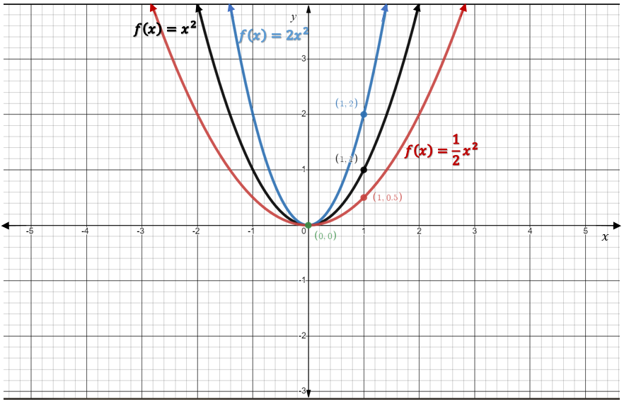
Graphically, we can see that when the leading coefficient is [latex]2[/latex], the parabola is stretched vertically, whereas when the leading coefficient is [latex]\frac{1}{2}[/latex], the parabola has been compressed vertically. This allows us to learn about the nature of a graph of a parabola when the leading coefficient is a value other than [latex]1[/latex]. In fact, the absolute value of [latex]a[/latex] dictates the vertical stretch or compression of the graph of a quadratic equation.
Quadratic Equations Vertical Stretch or Compression
For a function of the form [latex]f(x)=ax^2[/latex],
if [latex]|a|>1[/latex], the function is stretched by a factor of [latex]a[/latex].
if [latex]|a|<1[/latex], the function is compressed by a factor of [latex]a[/latex].
Another way to observe the effects of vertical stretches and compressions is in the table of values associated with a particular function. For example, let’s compare the table of values for the functions [latex]f(x)=x^2[/latex] and [latex]f(x)=2x^2[/latex]. You will see that the [latex]y[/latex]-values of the graph of [latex]f(x)=2x^2[/latex] have been multiplied by [latex]2[/latex] and these values are reflected in Figure 5.7.2.
| [latex]x[/latex] | [latex]f(x)=x^2[/latex] |
|---|---|
| [latex]-2[/latex] | [latex]4[/latex] |
| [latex]-1[/latex] | [latex]1[/latex] |
| [latex]0[/latex] | [latex]0[/latex] |
| [latex]1[/latex] | [latex]1[/latex] |
| [latex]2[/latex] | [latex]4[/latex] |
| [latex]x[/latex] | [latex]f(x)=2x^2[/latex] |
|---|---|
| [latex]-2[/latex] | [latex]8[/latex] |
| [latex]-1[/latex] | [latex]2[/latex] |
| [latex]0[/latex] | [latex]0[/latex] |
| [latex]1[/latex] | [latex]2[/latex] |
| [latex]2[/latex] | [latex]8[/latex] |
Finally, let’s examine what happens when we add a vertical translation of [latex]k[/latex] to the quadratic equation. In the figure below (Figure 5.7.3), we see graphs of the equations [latex]f(x)=x^2[/latex], [latex]f(x)=x^2+2[/latex], and [latex]f(x)=x^2-2[/latex].
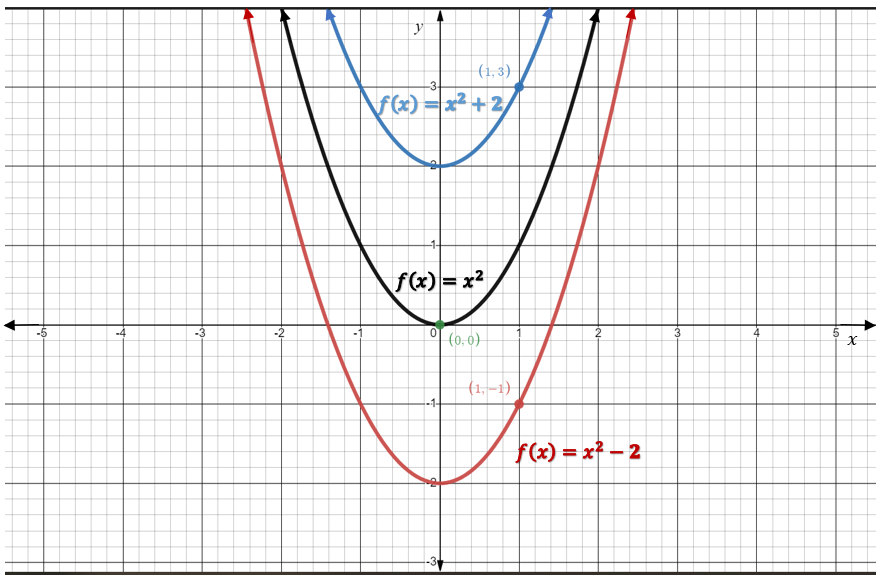
Graphically, we can see that a vertical translation either moves the parabola up by [latex]k[/latex] units or down by [latex]|k|[/latex] units.
Once again, we can also see these transformations within the table of values associated with the given functions. Below, we compare [latex]f(x)=x^2[/latex] to [latex]f(x)=x^2-2[/latex]. We see that the [latex]y[/latex]-values have all been reduced by [latex]2[/latex]. It is also important to notice that the [latex]y[/latex]-intercept (vertex) was also shifted down by [latex]2[/latex] units.
| [latex]x[/latex] | [latex]f(x)=x^2[/latex] |
|---|---|
| [latex]-2[/latex] | [latex]4[/latex] |
| [latex]-1[/latex] | [latex]1[/latex] |
| [latex]0[/latex] | [latex]0[/latex] |
| [latex]1[/latex] | [latex]1[/latex] |
| [latex]2[/latex] | [latex]4[/latex] |
| [latex]x[/latex] | [latex]f(x)=x^2-2[/latex] |
|---|---|
| [latex]-2[/latex] | [latex]2[/latex] |
| [latex]-1[/latex] | [latex]-1[/latex] |
| [latex]0[/latex] | [latex]-2[/latex] |
| [latex]1[/latex] | [latex]-1[/latex] |
| [latex]2[/latex] | [latex]2[/latex] |
Quadratic Equations Vertical Translation
For a function of the form [latex]f(x)=ax^2+k[/latex],
if [latex]k>0[/latex], the function is translated up by [latex]k[/latex] units.
if [latex]k<0[/latex], the function is translated down by [latex]|k|[/latex] units.
HOW TO
Graph a polynomial function of the form [latex]f(x)=ax^2+k[/latex].
- Find the direction of opening by observing the sign of [latex]a[/latex].
- Find the [latex]y[/latex]-intercept, which is also the vertex, by setting [latex]x=0[/latex] and evaluating for [latex]y[/latex].
- Make a table of values for [latex]-2\le x\le 2[/latex].
- Plot the vertex and the ordered pairs from the table of values.
- Join the points by a curve. Be sure to make the curve smooth with no sharp edges or points.
- Remember the rules of good graphing (label axes, arrows on ends of axes and curves, at least [latex]3[/latex] scale markings in each relevant, and original equations labelled).
Example 5.7.1
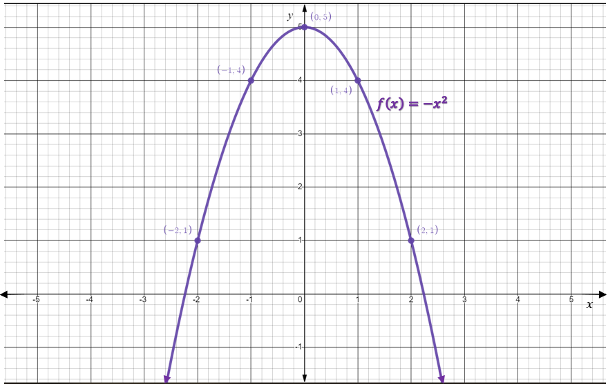
Graph the function [latex]f(x)=-x^2+5[/latex].
Solution
Step 1: Note that the leading coefficient [latex]a=-1[/latex]. This means that the parabola will open downwards.
Step 2: The [latex]y[/latex]-intercept can be found by setting [latex]x=0[/latex], and evaluating for the value of the function.
[latex]\begin{eqnarray*}f(x)&=&-x^2+5\\f(0)&=&-(0)^2+5\\f(0)&=&5\end{eqnarray*}[/latex]
Therefore, the [latex]y[/latex]-intercept is the point [latex](0,5)[/latex]
Step 3: Make a table of values for [latex]-2\le x\le 2[/latex].
| [latex]x[/latex] | [latex]f(x)=-x^2+5[/latex] |
|---|---|
| [latex]-2[/latex] | [latex]1[/latex] |
| [latex]-1[/latex] | [latex]4[/latex] |
| [latex]0[/latex] | [latex]5[/latex] |
| [latex]1[/latex] | [latex]4[/latex] |
| [latex]2[/latex] | [latex]1[/latex] |
Step 4: Plot the vertex and the ordered pairs from the table of values.
Step 5: Join the points by a curve. Be sure to make the curve smooth with no sharp edges or points.
Step 6: Remember the rules of good graphing (label axes, arrows on ends of axes and curves, at least [latex]3[/latex] scale markings in each relevant, and original equations labelled).
Example 5.7.2
Graph the function [latex]f(x)=2x^2-4[/latex].
Solution
Step 1: Note that the leading coefficient [latex]a=2[/latex]. This means that the parabola will open downwards.
Step 2: The [latex]y[/latex]-intercept can be found by setting [latex]x=0[/latex], and evaluating for the value of the function.
[latex]\begin{eqnarray*}f(x)&=&2x^2-4\\f(0)&=&2(0)^2-4\\f(0)&=&-4\end{eqnarray*}[/latex]
Therefore, the [latex]y[/latex]-intercept is the point [latex](0,-4)[/latex]
Step 3: Make a table of values for [latex]-2\le x\le 2[/latex].
| [latex]x[/latex] | [latex]f(x)=2x^2-4[/latex] |
|---|---|
| [latex]-2[/latex] | [latex]4[/latex] |
| [latex]-1[/latex] | [latex]-2[/latex] |
| [latex]0[/latex] | [latex]-4[/latex] |
| [latex]1[/latex] | [latex]-2[/latex] |
| [latex]2[/latex] | [latex]4[/latex] |
Step 4: Plot the vertex and the ordered pairs from the table of values.
Step 5: Join the points by a curve. Be sure to make the curve smooth with no sharp edges or points.
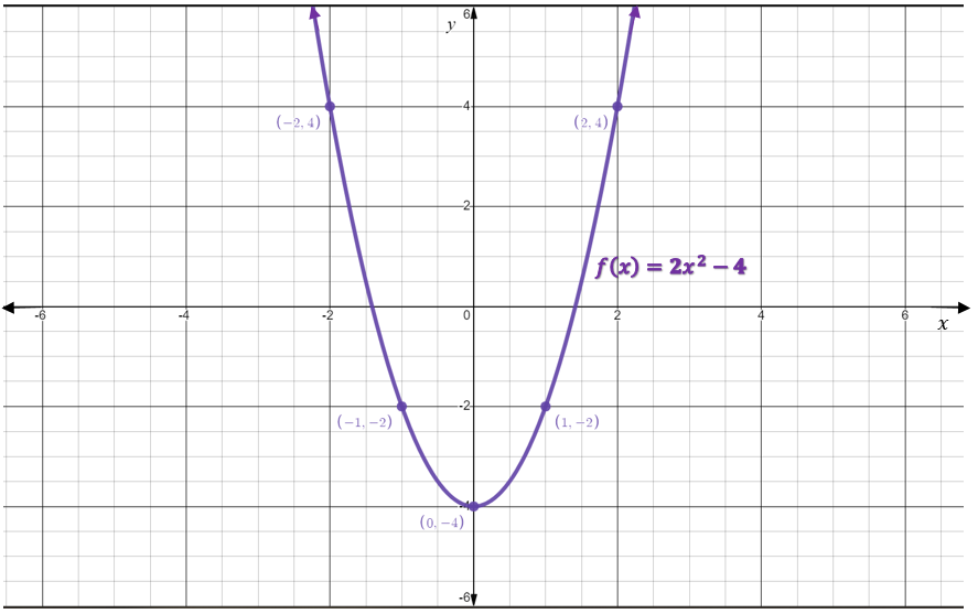
Step 6: Remember the rules of good graphing (label axes, arrows on ends of axes and curves, at least [latex]3[/latex] scale markings in each relevant, and original equations labelled).
Try It
Graphs of Cubic Equations
A cubic equation is one that contains a cubed variable term. In this section, we will focus on the graphs of cubic equations of the form [latex]f(x)=ax^3+k[/latex]. It is important to note that cubic equations can have graphs that do not have this general shape, but we restrict our focus to cubic equations whose graphs have not undergone any further transformations other than vertical reflections and translations. We will see that changing the leading coefficient and the value of [latex]k[/latex] will affect the graphs of cubic equations in the same (or similar) way as those transformations affected the graphs of quadratic equations.
Let’s begin by comparing the graphs of the equations [latex]f(x)=x^3[/latex] and [latex]f(x)=-x^3[/latex].
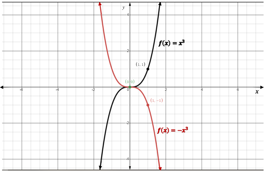
As we can see above, the only difference between the two graphs is their orientation, and the only difference between the equations is the sign of the leading coefficient, [latex]a[/latex]. When [latex]a[/latex] is positive ([latex]a>0[/latex]), the graph increases initially and for all of the values of [latex]x[/latex]. Contrarily, when [latex]a[/latex] is negative ([latex]a<0[/latex]), the graph decreases initially and for all of the values of [latex]x[/latex]. It is important to note that some cubic functions do have intervals of both increase and decrease, but since we are only studying cubic equations of the form [latex]f(x)=ax^3+k[/latex], we will not investigate that case.
Cubic Equations Direction of Increase or Decrease
For cubic equations of the form [latex]f(x)=ax^3+k[/latex],
If [latex]a>0[/latex], the function is increasing for all values of [latex]x[/latex].
If [latex]a<0[/latex], the function is decreasing for all values of [latex]x[/latex].
We can also make note that the [latex]y[/latex]-intercept of these graphs is the origin, [latex](0,0)[/latex]. In the case of cubic equations of this particular form, the [latex]y[/latex]-intercept is also the point of inflection. An inflection point is a point where a curve changes its concavity.
Next, we’ll examine the graphs [latex]f(x)=2x^3[/latex] and [latex]f(x)=\frac{1}{2}x^3[/latex], alongside [latex]f(x)=x^3[/latex] for comparison. The figure below shows that cubic equations can undergo vertical stretches and compressions in the same way that quadratic equations could.
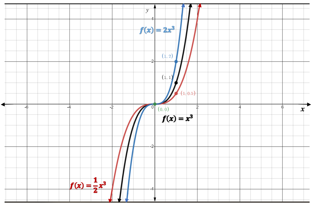
Cubic Equations Vertical Stretch and Compression
For a function of the form [latex]f(x)=ax^3[/latex],
if [latex]|a|>1[/latex], the function is stretched by a factor of [latex]a[/latex].
if [latex]|a|<1[/latex], the function is compressed by a factor of [latex]a[/latex].
What do we think would happen if we added a vertical translation to the equation? What might that look like? As was the case with quadratic equations, the graphs of cubic equations behave in the same way when they undergo vertical translations. The following figure show the graphs of [latex]f(x)=x^3[/latex], [latex]f(x)=x^3+2[/latex] and [latex]f(x)=x^3-2[/latex].
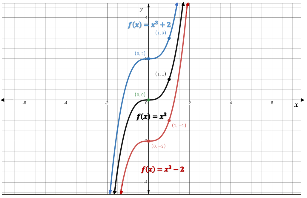
Cubic Equations Vertical Translation
For a function of the form [latex]f(x)=ax^3+k[/latex],
if [latex]k>0[/latex], the function is translated up by [latex]k[/latex] units.
if [latex]k<0[/latex], the function is translated down by [latex]|k|[/latex] units.
If we were to make a table of values for the cubic equations [latex]f(x)=x^3[/latex] and [latex]f(x)=x^3-3[/latex], we would see that the [latex]y[/latex]-values have been reduced by [latex]3[/latex].
| [latex]x[/latex] | [latex]f(x)=x^3[/latex] |
|---|---|
| [latex]-2[/latex] | [latex]-8[/latex] |
| [latex]-1[/latex] | [latex]-1[/latex] |
| [latex]0[/latex] | [latex]0[/latex] |
| [latex]1[/latex] | [latex]1[/latex] |
| [latex]2[/latex] | [latex]8[/latex] |
| [latex]x[/latex] | [latex]f(x)=x^3-3[/latex] |
|---|---|
| [latex]-2[/latex] | [latex]-11[/latex] |
| [latex]-1[/latex] | [latex]-4[/latex] |
| [latex]0[/latex] | [latex]-3[/latex] |
| [latex]1[/latex] | [latex]-2[/latex] |
| [latex]2[/latex] | [latex]5[/latex] |
Try It
3) Make a table of values for the functions [latex]f(x)=x^3[/latex] and [latex]f(x)=x^3+7[/latex] for [latex]-2\le x\le 2[/latex]. What transformation has occurred?
Solution
A translation of seven units upwards.
| [latex]x[/latex] | [latex]f(x)=x^3[/latex] |
|---|---|
| [latex]-2[/latex] | [latex]-8[/latex] |
| [latex]-1[/latex] | [latex]-1[/latex] |
| [latex]0[/latex] | [latex]0[/latex] |
| [latex]1[/latex] | [latex]1[/latex] |
| [latex]2[/latex] | [latex]8[/latex] |
| [latex]x[/latex] | [latex]f(x)=x^3+7[/latex] |
|---|---|
| [latex]-2[/latex] | [latex]-1[/latex] |
| [latex]-1[/latex] | [latex]6[/latex] |
| [latex]0[/latex] | [latex]7[/latex] |
| [latex]1[/latex] | [latex]8[/latex] |
| [latex]2[/latex] | [latex]15[/latex] |
HOW TO
Graph a polynomial function of the form [latex]f(x)=ax^3+k[/latex].
- Find the direction of the curve by observing the sign of [latex]a[/latex].
- Find the [latex]y[/latex]-intercept, which is also the inflection point, by setting [latex]x=0[/latex] and evaluating for [latex]y[/latex].
- Make a table of values for [latex]-2\le x\le 2[/latex].
- Plot the [latex]y[/latex]-intercept and the ordered pairs from the table of values.
- Join the points by a curve. Be sure to make the curve smooth with no sharp edges or points.
- Remember the rules of good graphing (label axes, arrows on ends of axes and curves, at least [latex]3[/latex] scale markings in each relevant direction, and original equations labelled).
Example 5.7.3
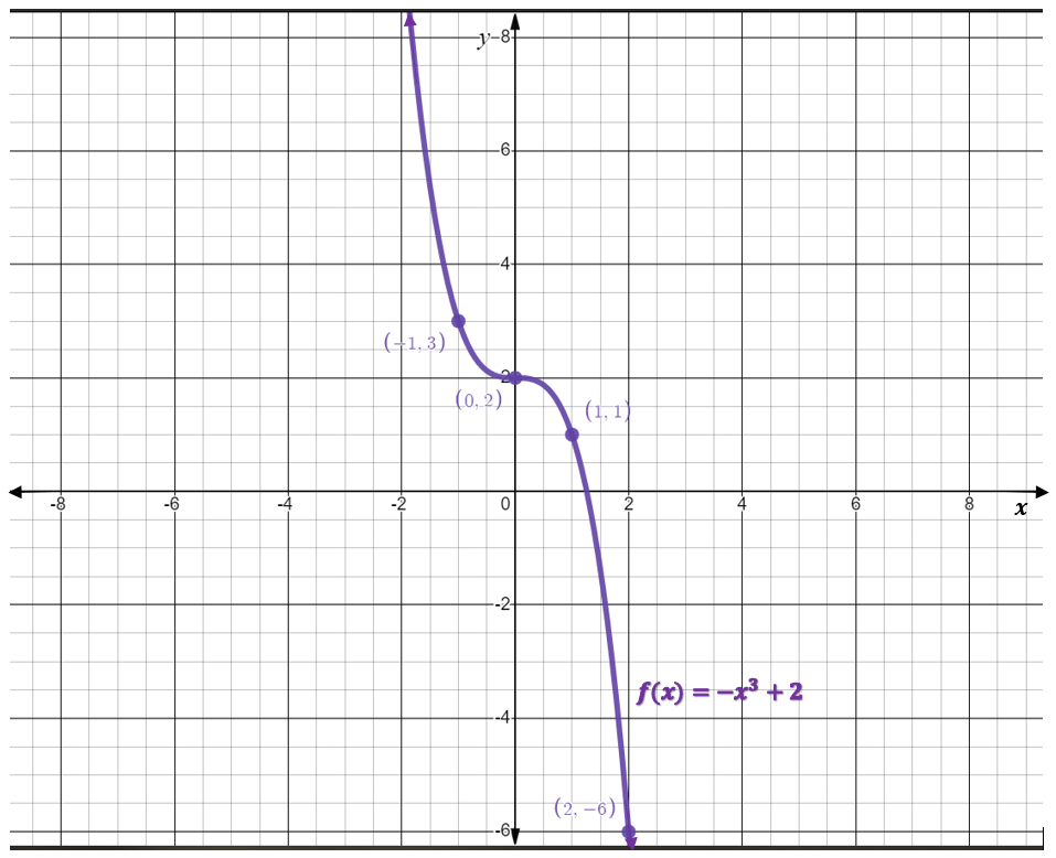
Graph the function [latex]f(x)=-x^3+2[/latex].
Solution
Step 1: Note that the leading coefficient [latex]a=-1[/latex]. This means that the graph of the cubic will be decreasing.
Step 2: The [latex]y[/latex]-intercept can be found by setting [latex]x=0[/latex], and evaluating for the value of the function.
[latex]\begin{eqnarray*}f(x)&=&-x^3+2\\f(0)&=&-(0)^3+2\\f(0)&=&2\end{eqnarray*}[/latex]
Therefore, the [latex]y[/latex]-intercept is the point [latex](0,2)[/latex]
Step 3: Make a table of values for [latex]-2\le x\le 2[/latex].
| [latex]x[/latex] | [latex]f(x)=-x^3+2[/latex] |
|---|---|
| [latex]-2[/latex] | [latex]10[/latex] |
| [latex]-1[/latex] | [latex]3[/latex] |
| [latex]0[/latex] | [latex]2[/latex] |
| [latex]1[/latex] | [latex]1[/latex] |
| [latex]2[/latex] | [latex]-6[/latex] |
Step 4: Plot the [latex]y[/latex]-intercept and the ordered pairs from the table of values.
Step 5: Join the points by a curve. Be sure to make the curve smooth with no sharp edges or points.
Step 6: Remember the rules of good graphing (label axes, arrows on ends of axes and curves, at least [latex]3[/latex] scale markings in each relevant, and original equations labelled).
Example 5.7.4
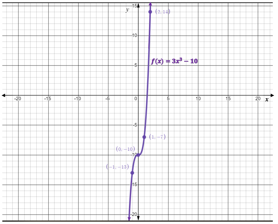
Graph the function [latex]f(x)=3x^3-10[/latex].
Solution
Step 1: Note that the leading coefficient [latex]a=3[/latex]. This means that the graph of the cubic will be increasing.
Step 2: The [latex]y[/latex]-intercept can be found by setting [latex]x=0[/latex], and evaluating for the value of the function.
[latex]\begin{eqnarray*}f(x)&=&3x^3-10\\f(0)&=&3(0)^3-10\\f(0)&=&-10\end{eqnarray*}[/latex]
Therefore, the [latex]y[/latex]-intercept is the point [latex](0,2)[/latex]
Step 3: Make a table of values for [latex]-2\le x\le 2[/latex].
| [latex]x[/latex] | [latex]f(x)=-x^3+2[/latex] |
|---|---|
| [latex]-2[/latex] | [latex]-34[/latex] |
| [latex]-1[/latex] | [latex]-13[/latex] |
| [latex]0[/latex] | [latex]-10[/latex] |
| [latex]1[/latex] | [latex]-7[/latex] |
| [latex]2[/latex] | [latex]14[/latex] |
Step 4: Plot the [latex]y[/latex]-intercept and the ordered pairs from the table of values.
Step 5: Join the points by a curve. Be sure to make the curve smooth with no sharp edges or points.
Step 6: Remember the rules of good graphing (label axes, arrows on ends of axes and curves, at least [latex]3[/latex] scale markings in each relevant, and original equations labelled).
Try It
Key Concepts
1) Quadratic Equations Direction of Opening
For a function of the form [latex]f(x)=ax^2[/latex],
if [latex]a>0[/latex], the parabola opens upwards;
if [latex]a<0[/latex], the parabola opens downwards.
2) Quadratic Equations Vertical Stretch or Compression
For a function of the form [latex]f(x)=ax^2[/latex],
if [latex]|a|>1[/latex], the function is stretched by a factor of [latex]a[/latex].
if [latex]|a|<1[/latex], the function is compressed by a factor of [latex]a[/latex].
3) Quadratic Equations Vertical Translation
For a function of the form [latex]f(x)=ax^2+k[/latex],
if [latex]k>0[/latex], the function is translated up by [latex]k[/latex] units.
if [latex]k<0[/latex], the function is translated down by [latex]|k|[/latex] units.
4) How To Graph a polynomial function of the form [latex]f(x)=ax^2+k[/latex].
-
- Find the direction of opening by observing the sign of [latex]a[/latex].
- Find the [latex]y[/latex]-intercept, which is also the vertex, by setting [latex]x=0[/latex] and evaluating for [latex]y[/latex].
- Make a table of values for [latex]-2\le x\le 2[/latex].
- Plot the vertex and the ordered pairs from the table of values.
- Join the points by a curve. Be sure to make the curve smooth with no sharp edges or points.
- Remember the rules of good graphing (label axes, arrows on ends of axes and curves, at least [latex]3[/latex] scale markings in each relevant, and original equations labelled).
5) Cubic Equations Direction of Increase or Decrease
For cubic equations of the form [latex]f(x)=ax^3+k[/latex],
If [latex]a>0[/latex], the function is increasing for all values of [latex]x[/latex].
If [latex]a<0[/latex], the function is decreasing for all values of [latex]x[/latex].
6) Cubic Equations Vertical Stretch and Compression
For a function of the form [latex]f(x)=ax^3[/latex],
if [latex]|a|>1[/latex], the function is stretched by a factor of [latex]a[/latex].
if [latex]|a|<1[/latex], the function is compressed by a factor of [latex]a[/latex].
7) Cubic Equations Vertical Translation
For a function of the form [latex]f(x)=ax^3+k[/latex],
if [latex]k>0[/latex], the function is translated up by [latex]k[/latex] units.
if [latex]k<0[/latex], the function is translated down by [latex]|k|[/latex] units.
8) How To Graph a polynomial function of the form [latex]f(x)=ax^3+k[/latex].
-
- Find the direction of the curve by observing the sign of [latex]a[/latex].
- Find the [latex]y[/latex]-intercept, which is also the inflection point, by setting [latex]x=0[/latex] and evaluating for [latex]y[/latex].
- Make a table of values for [latex]-2\le x\le 2[/latex].
- Plot the [latex]y[/latex]-intercept and the ordered pairs from the table of values.
- Join the points by a curve. Be sure to make the curve smooth with no sharp edges or points.
- Remember the rules of good graphing (label axes, arrows on ends of axes and curves, at least [latex]3[/latex] scale markings in each relevant direction, and original equations labelled).
Self Check
After completing the exercises, use this checklist to evaluate your mastery of the objectives of this section.
Overall, after looking at the checklist, do you think you are well-prepared for the next section? Why or why not?
