2.2 Accuracy, Precision, and Rounding Rules
Learning Objectives
By the end of this section, you will be able to:
- Identify exact and inexact numbers.
- Recognize the number of significant figures in a given quantity.
- Identify the number of decimal places.
- Understand the difference between accuracy and precision.
- Calculate the percent uncertainty of a measurement.
- Apply the concept of significant figures to limit mathematical results to the proper number of digits.
Exact and Inexact Numbers
When considering measurement, we must consider the nature of the numbers that we are using in our calculations.
A number is exact if it is known with complete certainty. An exact number is a number that you can get by counting. Exact numbers have infinitely many significant figures and decimal places. For example, there are exactly 100 centimeters in one meter and exactly 4 quarts in a gallon.
A number is inexact if it has uncertainty associated with it. This uncertainty can arise due to measurement or rounding. Some examples would be a person’s height or weight.
Accuracy and Precision of a Measurement
Science is based on observation and experiment—that is, on measurements. Accuracy is how close a measurement is to the correct value for that measurement. For example, let us say that you are measuring the length of standard computer paper. The packaging in which you purchased the paper states that it is 11.0 inches long. You measure the length of the paper three times and obtain the following measurements: 11.1 in., 11.2 in., and 10.9 in. These measurements are quite accurate because they are very close to the correct value of 11.0 inches. In contrast, if you had obtained a measurement of 12 inches, your measurement would not be very accurate.
The precision of a measurement system is refers to how close the agreement is between repeated measurements (which are repeated under the same conditions). Consider the example of the paper measurements. The precision of the measurements refers to the spread of the measured values. One way to analyze the precision of the measurements would be to determine the range, or difference, between the lowest and the highest measured values. In that case, the lowest value was 10.9 in. and the highest value was 11.2 in. Thus, the measured values deviated from each other by at most 0.3 in. These measurements were relatively precise because they did not vary too much in value. However, if the measured values had been 10.9, 11.1, and 11.9, then the measurements would not be very precise because there would be significant variation from one measurement to another.
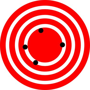
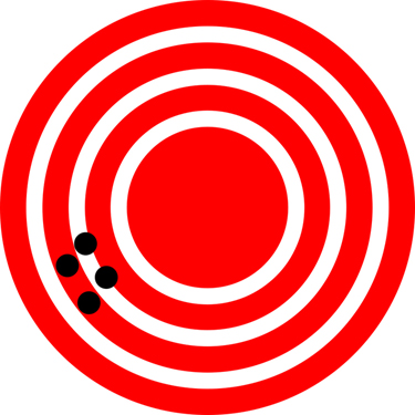
The measurements in the paper example are both accurate and precise, but in some cases, measurements are accurate but not precise, or they are precise but not accurate. Let us consider an example of a GPS system that is attempting to locate the position of a restaurant in a city. Think of the restaurant location as existing at the centre of a bull’s-eye target, and think of each GPS attempt to locate the restaurant as a black dot. In Figure 2.2.1 you can see that the GPS measurements are spread out far apart from each other, but they are all relatively close to the actual location of the restaurant at the centre of the target. This indicates a low precision, high accuracy measuring system. However, in Figure 2.2.2 the GPS measurements are concentrated quite closely to one another, but they are far away from the target location. This indicates a high precision, low accuracy measuring system.
Accuracy, Precision, and Uncertainty
The degree of accuracy and precision of a measuring system are related to the uncertainty in the measurements. Uncertainty is a quantitative measure of how much your measured values deviate from a standard or expected value. If your measurements are not very accurate or precise, then the uncertainty of your values will be very high. In more general terms, uncertainty can be thought of as a disclaimer for your measured values. For example, if someone asked you to provide the mileage on your car, you might say that it is 45,000 miles, plus or minus 500 miles. The plus or minus amount is the uncertainty in your value. That is, you are indicating that the actual mileage of your car might be as low as 44,500 miles or as high as 45,500 miles, or anywhere in between. All measurements contain some amount of uncertainty. In our example of measuring the length of the paper, we might say that the length of the paper is 11 in., plus or minus 0.2 in. The uncertainty in a measurement, [latex]A[/latex], is often denoted as [latex]\delta A[/latex] (“delta [latex]A[/latex]”), so the measurement result would be recorded as [latex]A\pm \delta A[/latex]. In our paper example, the length of the paper could be expressed as [latex]11 in. \pm 0.2[/latex].
The factors contributing to uncertainty in a measurement include:
- Limitations of the measuring device,
- The skill of the person making the measurement,
- Irregularities in the object being measured,
- Any other factors that affect the outcome (highly dependent on the situation).
In our example, such factors contributing to the uncertainty could be the following: the smallest division on the ruler is 0.1 in., the person using the ruler has bad eyesight, or one side of the paper is slightly longer than the other. At any rate, the uncertainty in a measurement must be based on a careful consideration of all the factors that might contribute and their possible effects.
Making Connections: Real World Connections – Fever or Chills?
Uncertainty is a critical piece of information, both in physics and in many other real-world applications. Imagine you are caring for a sick child. You suspect the child has a fever, so you check his or her temperature with a thermometer. What if the uncertainty of the thermometer were 3.0 °C? If the child’s temperature reading was 37.0 °C (which is normal body temperature), the “true” temperature could be anywhere from a hypothermic 34.0 °C to a dangerously high 40.0 °C. A thermometer with an uncertainty of 3.0 °C would be useless.
Percent Uncertainty
One method of expressing uncertainty is as a percent of the measured value. If a measurement [latex]A[/latex] is expressed with [latex]uncertainty[/latex], [latex]\delta A[/latex], the percent uncertainty (%unc) is defined to be:
Example 2.2.1
A grocery store sells 5-lb bags of apples. You purchase four bags over the course of a month and weigh the apples each time. You obtain the following measurements:
- Week 1 weight: 4.8 lb
- Week 2 weight: 5.3 lb
- Week 3 weight: 4.9 lb
- Week 4 weight: 5.4 lb
You determine that the weight of the 5-lb bag has an uncertainty of ±0.4 lb. What is the percent uncertainty of the bag’s weight?
Strategy
First, observe that the expected value of the bag’s weight, [latex]A[/latex], is 5 lb. The uncertainty in this value, [latex]\delta A[/latex], is 0.4 lb. We can use the following equation to determine the percent uncertainty of the weight:
Solution
Plug the known values into the equation:
Discussion
We can conclude that the weight of the apple bag is 5 lb ±8%. Consider how this percent uncertainty would change if the bag of apples were half as heavy, but the uncertainty in the weight remained the same. Hint for future calculations: when calculating percent uncertainty, always remember that you must multiply the fraction by 100%. If you do not do this, you will have a decimal quantity, not a percent value.
Uncertainties in Calculations
There is an uncertainty in anything calculated from measured quantities. For example, the area of a floor calculated from measurements of its length and width has an uncertainty because the length and width have uncertainties. How big is the uncertainty in something you calculate by multiplication or division? If the measurements going into the calculation have small uncertainties (a few percent or less), then the method of adding percents can be used for multiplication or division. This method says that the percent uncertainty in a quantity calculated by multiplication or division is the sum of the percent uncertainties in the items used to make the calculation. For example, if a floor has a length of 4.00 m and a width of 3.00 m, with uncertainties of 2% and 1%, respectively, then the area of the floor is 12.0 m and has an uncertainty of 3%. (Expressed as an area this is 0.36 m2, which we round to 0.4 m2 since the area of the floor is given to a tenth of a square meter.)
Try It
1) A high school track coach has just purchased a new stopwatch. The stopwatch manual states that the stopwatch has an uncertainty of ±0.05 s. Runners on the track coach’s team regularly clock 100-m sprints of 11.49 s to 15.01 s. At the school’s last track meet, the first-place sprinter came in at 12.04 s and the second-place sprinter came in at 12.07 s. Will the coach’s new stopwatch be helpful in timing the sprint team? Why or why not?
Solution
No, the uncertainty in the stopwatch is too great to effectively differentiate between the sprint times.
Precision of Measuring Tools and Significant Figures
An important factor in the accuracy and precision of measurements involves the precision of the measuring tool. In general, a precise measuring tool is one that can measure values in very small increments. For example, a standard ruler can measure length to the nearest millimeter, while a caliper can measure length to the nearest 0.01 millimeter. The caliper is a more precise measuring tool because it can measure extremely small differences in length. The more precise the measuring tool, the more precise and accurate the measurements can be.
When we express measured values, we can only list as many digits as we initially measured with our measuring tool. For example, if you use a standard ruler to measure the length of a stick, you may measure it to be 36.7 cm. You could not express this value as 36.71 cm because your measuring tool was not precise enough to measure a hundredth of a centimeter. It should be noted that the last digit in a measured value has been estimated in some way by the person performing the measurement. For example, the person measuring the length of a stick with a ruler notices that the stick length seems to be somewhere in between 36.6 cm and 36.7 cm, and he or she must estimate the value of the last digit. Using the method of significant figures, the rule is that the last digit written down in a measurement is the first digit with some uncertainty. In order to determine the number of significant digits in a value, start with the first measured value at the left and count the number of digits through the last digit written on the right. For example, the measured value 36.7 cm has three digits, or significant figures. Significant figures indicate the precision of a measuring tool that was used to measure a value.
Significant Figures: Zeros
Special consideration is given to zeros when counting significant figures. The zeros in 0.053 are not significant, because they are only placekeepers that locate the decimal point. There are two significant figures in 0.053. The zeros in 10.053 are not placekeepers but are significant—this number has five significant figures. The zeros in 1300 may or may not be significant depending on the style of writing numbers. They could mean the number is known to the last digit, or they could be placekeepers. So 1300 could have two, three, or four significant figures. (To avoid this ambiguity, write 1300 in scientific notation.) Zeros are significant except when they serve only as placekeepers.
Try It
2) Determine the number of significant figures in the following measurements:
a) 0.0009
b) 15,450.0
c) 6×10³
d) 87.990
e) 30.42
Solution
a) 1
b) 6
c) 1
d) 5
e) 4
As you have probably realized by now, the biggest issue in determining the number of significant figures in a value is the zero. Is the zero significant or not? One way to unambiguously determine whether a zero is significant or not is to write a number in scientific notation. Scientific notation will include zeros in the coefficient of the number only if they are significant. Thus, the number 8.666 × 10⁶ has four significant figures. However, the number 8.6660 × 10⁶ has five significant figures. That last zero is significant; if it were not, it would not be written in the coefficient. So when in doubt about expressing the number of significant figures in a quantity, use scientific notation and include the number of zeros that are truly significant. We will learn more about scientific notation in a later section in the text.
Significant Figures
If you use a calculator to evaluate the expression [latex]\frac{337}{217}[/latex], you will get the following:
[latex]\frac{337}{217}=1.55299539171...[/latex]
and so on for many more digits. Although this answer is correct, it is somewhat presumptuous. You start with two values that each have three digits, and the answer has twelve digits? That does not make much sense from a strict numerical point of view.
Consider using a ruler to measure the width of an object, as shown in Figure 2.2.3 “Expressing Width”. The object is definitely more than 1 cm long, so we know that the first digit in our measurement is 1. We see by counting the tick marks on the ruler that the object is at least three ticks after the 1. If each tick represents 0.1 cm, then we know the object is at least 1.3 cm wide. But our ruler does not have any more ticks between the 0.3 and the 0.4 marks, so we can’t know exactly how much the next decimal place is. But with a practised eye we can estimate it. Let us estimate it as about six-tenths of the way between the third and fourth tick marks, which estimates our hundredths place as 6, so we identify a measurement of 1.36 cm for the width of the object.
What is the proper way to express the width of this object?
Does it make any sense to try to report a thousandths place for the measurement? No, it doesn’t; we are not exactly sure of the hundredths place (after all, it was an estimate only), so it would be fruitless to estimate a thousandths place. Our best measurement, then, stops at the hundredths place, and we report 1.36 cm as proper measurement.
This concept of reporting the proper number of digits in a measurement or a calculation is called significant figures. Significant figures (sometimes called significant digits) represent the limits of what values of a measurement or a calculation we are sure of. The convention for a measurement is that the quantity reported should be all known values and the first estimated value. The conventions for calculations are discussed as follows.
Example 2.2.2
Use each diagram to report a measurement to the proper number of significant figures.
-
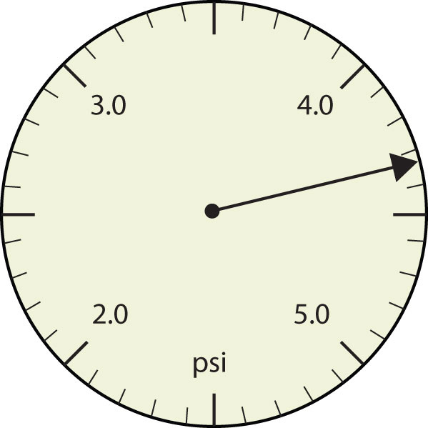
Figure 2.2.4. Pressure gauge in units of pounds per square inch -
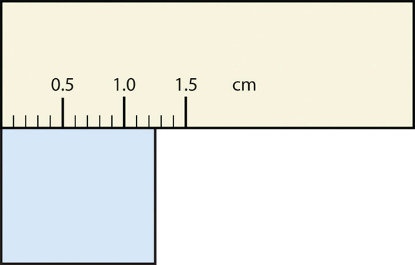
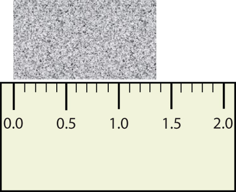
Figure 2.2.5. A measuring ruler

Solution
- The arrow is between 4.0 and 5.0, so the measurement is at least 4.0. The arrow is between the third and fourth small tick marks, so it’s at least 0.3. We will have to estimate the last place. It looks like about one-third of the way across the space, so let us estimate the hundredths place as 3. Combining the digits, we have a measurement of 4.33 psi (psi stands for “pounds per square inch” and is a unit of pressure, like air in a tire). We say that the measurement is reported to three significant figures.
- The rectangle is at least 1.0 cm wide but certainly not 2.0 cm wide, so the first significant digit is 1. The rectangle’s width is past the second tick mark but not the third; if each tick mark represents 0.1, then the rectangle is at least 0.2 in the next significant digit. We have to estimate the next place because there are no markings to guide us. It appears to be about halfway between 0.2 and 0.3, so we will estimate the next place to be a 5. Thus, the measured width of the rectangle is 1.25 cm. Again, the measurement is reported to three significant figures
Try It
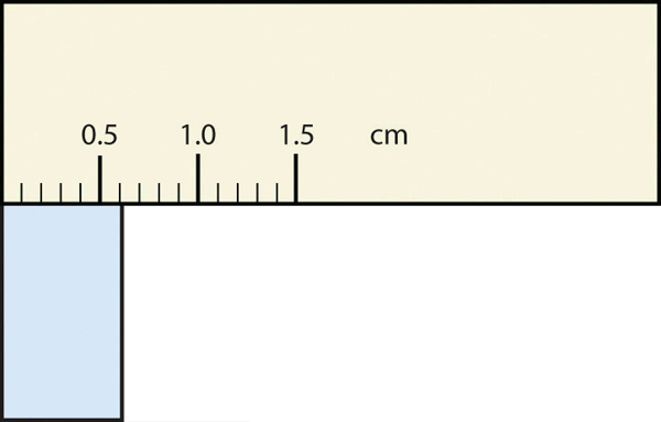
3) What would be the reported width of this rectangle?
Solution
0.63cm
In many cases, you will be given a measurement. How can you tell by looking what digits are significant? For example, the reported population of the United States is 306,000,000. Does that mean that it is exactly three hundred six million or is some estimation occurring?
The following conventions dictate which numbers in a reported measurement are significant and which are not significant:
- Any nonzero digit is significant.
- Any zeros between nonzero digits (i.e., embedded zeros) are significant.
- Zeros at the end of a number:
- without a decimal point (i.e., trailing zeros) are not significant; they serve only to put the significant digits in the correct positions.
- with a decimal point are significant.
- Zeros at the beginning of a decimal number (i.e., leading zeros) are not significant; again, they serve only to put the significant digits in the correct positions.
So, by these rules, the population figure of the United States has only three significant figures: the 3, the 6, and the zero between them. The remaining six zeros simply put the 306 in the millions position.
Example 2.2.3
Give the number of significant figures in each measurement.
- 36.7 m
- 0.006606 s
- 2,002 kg
- 306,490,000 people
Solution
- By rule 1, all nonzero digits are significant, so this measurement has three significant figures.
- By rule 4, the first three zeros are not significant, but by rule 2 the zero between the sixes is; therefore, this number has four significant figures.
- By rule 2, the two zeros between the twos are significant, so this measurement has four significant figures.
- The four trailing zeros in the number are not significant, but the other five numbers are, so this number has five significant figures.
Try It
Give the number of significant figures in each measurement.
4) 0.000601 m
Solution
[latex]3[/latex] significant figures
5) 65.080 kg
Solution
[latex]5[/latex] significant figures
Significant Figures in Calculations
How are significant figures handled in calculations? It depends on what type of calculation is being performed. If the calculation is an addition or a subtraction, the rule is as follows: limit the reported answer to the rightmost column that all numbers have significant figures in common. For example, if you were to add 1.2 and 4.71, we note that the first number stops its significant figures in the tenths column, while the second number stops its significant figures in the hundredths column. We therefore limit our answer to the tenths column.
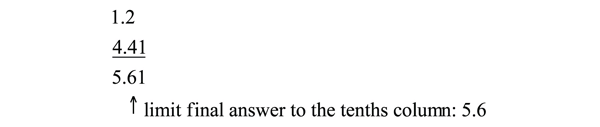
We drop the last digit—the 1—because it is not significant to the final answer.
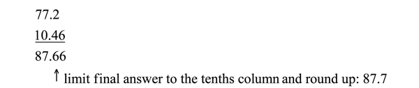
The dropping of positions in sums and differences brings up the topic of rounding. Although there are several conventions, in this text we will adopt the following rule: the final answer should be rounded up if the first dropped digit is 5 or greater and rounded down if the first dropped digit is less than 5.
Example 2.2.4
Express the final answer to the proper number of significant figures.
- [latex]101.2 + 18.702 = ?[/latex]
- [latex]202.88 − 1.013= ?[/latex]
Solution
- If we use a calculator to add these two numbers, we would get 119.902. However, most calculators do not understand significant figures, and we need to limit the final answer to the tenths place. Thus, we drop the 02 and report a final answer of 119.9 (rounding down).
- A calculator would answer 201.867. However, we have to limit our final answer to the hundredths place. Because the first number being dropped is 7, which is greater than 7, we round up and report a final answer of 201.87.
Try It
6) Express the answer for [latex]3.445 + 90.83 − 72.4[/latex] to the proper number of significant figures.
Solution
[latex]21.9[/latex]
If the operations being performed are multiplication or division, the rule is as follows: limit the answer to the number of significant figures that the data value with the least number of significant figures has. So if we are dividing 23 by 448, which have two and three significant figures each, we should limit the final reported answer to two significant figures (the lesser of two and three significant figures):
[latex]\frac{23}{448}=0.051339286...=0.051[/latex]
The same rounding rules apply in multiplication and division as they do in addition and subtraction.
Example 2.2.5
Express the final answer to the proper number of significant figures.
- [latex]76.4 \times 180.4 = ?[/latex]
- [latex]934.9\div 0.00455 = ?[/latex]
Solution
a. The first number has three significant figures, while the second number has four significant figures. Therefore, we limit our final answer to three significant figures:
[latex]76.4 \times 180.4 = 13,782.56 = 13,800[/latex].
b. The first number has four significant figures, while the second number has three significant figures. Therefore we limit our final answer to three significant figures:
[latex]934.9 \div 0.00455 = 205,472.5275… = 205,000[/latex].
Try It
Express the final answer to the proper number of significant figures.
7) [latex]22.4 \times 8.314 =[/latex]?
Solution
186
8) [latex]1.381 \div 6.02 =[/latex] ?
Solution
0.229
Example 2.2.6
Express the final answer to the proper number of significant figures.
- [latex](93.29-19.2) \times {1.2} = ?[/latex]
- [latex]810.0 \div {2.43 + 2.4} = ?[/latex]
Solution
- By the order of operations, we need to perform the subtraction first. Calculating this result would give 74.09 but we can only give our answer to the nearest tenth, so we need to round to 74.1. Then, we need to multiply 74.1 by 1.2 which gives 88.92 and we need to report this answer with two significant figures. Our answer is 89.
- By the order of operations, we need to perform the division first. This gives us [latex]333.\bar{3}[/latex]. Since 2.43 only has 3 significant figures, we need to limit our result to 3 significant figures, which gives us 333. Then, we need to add 2.4 to get 335.4. Finally, we need to give our answer to the nearest unit, and so our answer is 335.
Summary
When combining measurements with different degrees of accuracy and precision, the number of significant digits in the final answer can be no greater than the number of significant digits in the least precise measured value. There are two different rules, one for multiplication and division and the other for addition and subtraction, as discussed below.
1. For multiplication and division: The result should have the same number of significant figures as the quantity having the least significant figures entering into the calculation. For example, the area of a circle can be calculated from its radius using [latex]A=\mathrm{πr}^2[/latex]. Let us see how many significant figures the area has if the radius has only two—say, [latex]r=1.2 m[/latex]. Then,
[latex]A=\mathrm{πr}^2=3.1415927\times\left(1.2\;\mathrm m\right)^2=4.5238934\;\mathrm m^2[/latex]
is what you would get using a calculator that has an eight-digit output. But because the radius has only two significant figures, it limits the calculated quantity to two significant figures or
even though [latex]\mathrm\pi[/latex] is good to at least eight digits.
2. For addition and subtraction: The answer can contain no more decimal places than the least precise measurement. Suppose that you buy 7.56-kg of potatoes in a grocery store as measured with a scale with precision 0.01 kg. Then you drop off 6.052-kg of potatoes at your laboratory as measured by a scale with precision 0.001 kg. Finally, you go home and add 13.7 kg of potatoes as measured by a bathroom scale with precision 0.1 kg. How many kilograms of potatoes do you now have, and how many significant figures are appropriate in the answer? The mass is found by simple addition and subtraction:
[latex]\begin{align*} 7.56kg &\\ -6.052kg &\\ \underline{+\;\;13.7kg }&\\ 15.208kg&=15.2kg \end{align*}[/latex]
Next, we identify the least precise measurement: 13.7 kg. This measurement is expressed to the 0.1 decimal place, so our final answer must also be expressed to the 0.1 decimal place. Thus, the answer is rounded to the tenths place, giving us 15.2 kg.
3. For mixed operations: Round according to the rules above while following the order of operations for the calculations required. For example, perform the following operations and round to the appropriate number of significant figures.
[latex](3.495+12.45)\div 2.4[/latex]
We must add the values within the parentheses first, giving us 15.945. However, 12.45 is only precise to the nearest hundredth and so we need to round this result to the nearest hundredth, giving us 15.95. Then, we need to divide that by 2.4, which yields [latex]6.6458\bar{3}[/latex]. Since 15.95 has fours significant figures, and 2.4 only has two significant figures, we must round the answer to two significant figures, 6.6.
Rounding in Practical Situations
It is important to note that the rounding rules above are the theoretical rules used in chemical and physical laboratory papers and results. In various health care professions, the precision of the measurement tool being used will often dictate how you would round your medication dosages. In this sense, it is important to understand these theoretical rules and be aware that in practical situations, you may be taught best practices to coincide with the measurement tools available to you.
Key Concepts:
- Accuracy of a measured value refers to how close a measurement is to the correct value. The uncertainty in a measurement is an estimate of the amount by which the measurement result may differ from this value.
- Precision of measured values refers to how close the agreement is between repeated measurements.
- The precision of a measuring tool is related to the size of its measurement increments. The smaller the measurement increment, the more precise the tool.
- Significant figures express the precision of a measuring tool.
- Significant figures in a quantity indicate the number of known values plus one place that is estimated.
-
The following conventions dictate which numbers in a reported measurement are significant and which are not significant:
- Any nonzero digit is significant.
- Any zeros between nonzero digits (i.e., embedded zeros) are significant.
- Zeros at the end of a number without a decimal point (i.e., trailing zeros) are not significant; they serve only to put the significant digits in the correct positions. However, zeros at the end of any number with a decimal point are significant.
- Zeros at the beginning of a decimal number (i.e., leading zeros) are not significant; again, they serve only to put the significant digits in the correct positions.
- When multiplying or dividing measured values, the final answer can contain only as many significant figures as the least precise value.
- When adding or subtracting measured values, the final answer cannot contain more decimal places than the least precise value.
- When performing mixed operations, round according to the rules for addition/subtraction and multiplication/division while using the order of operations.
Self Check
After completing the exercises, use this checklist to evaluate your mastery of the objectives of this section.
Overall, after looking at the checklist, do you think you are well-prepared for the next section? Why or why not?
Glossary
- accuracy
- the degree to which a measure value agrees with the correct value for that measurement
- method of adding percents
- the percent uncertainty in a quantity calculated by multiplication or division is the sum of the percent uncertainties in the items used to make the calculation
- percent uncertainty
- the ratio of the uncertainty of a measurement to the measured value, expressed as a percentage
- precision
- the degree to which repeated measurements agree with each other
- significant figures
- express the precision of a measuring tool used to measure a value
- uncertainty
- a quantitative measure of how much your measured values deviate from a standard or expected value
a quantitative measure of how much your measured values deviate from a standard or expected value
the degree to which a measure value agrees with the correct value for that measurement
the degree to which repeated measurements agree with each other
the ratio of the uncertainty of a measurement to the measure value, express as a percentage
the percent uncertainty in a quantity calculated by multiplication or division is the sum of the percent uncertainties in the items used to make the calculation
the degree to which repeated measurements agree with each other
