Gradient of a function

L. El Ghaoui

Gradient of a function

The gradient of a differentiable function $f:\mathbb{R}^n \rightarrow \mathbb{R}$ contains the first derivatives of the function with respect to each variable. As seen here, the gradient is useful to find the linear approximation of the function near a point.

Definition
Composition rule
Examples
Geometric interpretation

Definition

The gradient of $f$ at $x_0$ , denoted $\nabla f(x_0)$ , is the vector in $R^n$ given by

$\nabla f\left(x_0\right)=\left(\begin{array}{c} \frac{\partial f}{\partial x_1}(x) \\ \vdots \\ \frac{\partial f}{\partial x_n}(x) \end{array}\right)$

Examples:

Distance function: The distance function from a point $p \in \mathbf{R}^2$ to another point $x \in \mathbf{R}^2$ is defined as

$\rho(x)=\|x-p\|_2=\sqrt{\left(x_1-p_1\right)^2+\left(x_2-p_2\right)^2} .$

The function is differentiable, provided $(x, y) \neq(p, q)$ , which we assume. Then

$\nabla \rho(x)=\frac{1}{\sqrt{\left(x_1-p_1\right)^2+\left(x_2-p_2\right)^2}}\left(\begin{array}{l} x_1-p_1 \\ x_2-p_2 \end{array}\right) .$

Log-sum-exp function: Consider the ‘‘log-sum-exp’’ function $lse: \mathbf{R}^2 \rightarrow \mathbf{R}$ , with values

$\operatorname{lse}(x):=\log \left(e^{x_1}+e^{x_2}\right) .$

The gradient of $L$ at $x$ is

$\nabla \operatorname{lse}(x)=\frac{1}{z_1+z_2}\left(\begin{array}{c} z_1 \\ z_2 \end{array}\right) .$

where $z_i:=e^{x_i}, i=1,2$ . More generally, the gradient of the function $lse: \mathbf{R}^n \rightarrow \mathbf{R}$ with values

$\operatorname{lse}(x)=\log \left(\sum_{i=1}^n e^{x_i}\right)$

is given by

$\nabla f(x)=\frac{1}{\sum_{i=1}^n e^{x_i}}\left(\begin{array}{c} e^{x_1} \\ \ldots \\ e^{x_n} \end{array}\right)=\frac{1}{Z} z,$

where $z=\left(e^{x_1}, \ldots, e^{x_n}\right)$ , and $Z=\sum_{i=1}^n z_i$ .

Composition rule with an affine function

If $A \in \mathbf{R}^{m \times n}$ is a matrix, and $b \in \mathbf{R}^m$ is a vector, the function $g: \mathbf{R}^m \rightarrow \mathbf{R}$ with values

$g(x)=f(A x+b)$

is called the composition of the affine map $x \rightarrow A x+b$ with $f$ with $f$ . Its gradient is given by (see here for proof)

$\nabla g(x)=A^T \nabla f(A x+b) .$

Geometric interpretation

Geometrically, the gradient can be read on the plot of the level set of the function. Specifically, at any point $x$ , the gradient is perpendicular to the level set and points outwards from the sub-level set (that is, it points towards higher values of the function).

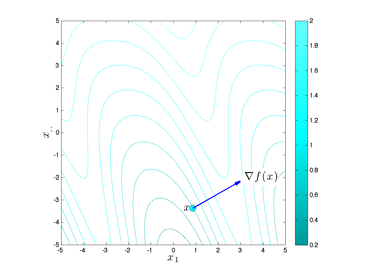Level and sub-level sets of the function $f:\mathbb{R}^n \rightarrow \mathbb{R}$ with values

$f(x) = lse(\sin(x_1 + 0,3 x_2), 0,2 x_2).$

The gradient at a point (shown in red) is perpendicular to the level set, and points outside the corresponding sub-level set. The length of the gradient determines how fast the function changes locally (The length of the gradient has been scaled up by a factor of $5$ .)

Gradient of a function

Definition

Composition rule with an affine function

Geometric interpretation

License

Share This Book