Basics
Basics
- Definitions
- Independence
- Subspaces, span, affine sets
- Basis, dimension
Definitions
Vectors
Assume we are given a collection of  real numbers,
  . We can represent them as locations on a line. Alternatively, we can represent the collection as a single point in a -dimensional space. This is the vector representation of the collection of numbers; each number
  is called a component or element of the vector.
Vectors can be arranged in a column or a row; we usually write vectors in column format:
(1) 
We denote by  denotes the set of real vectors with components. If
  denotes a vector, we use subscripts to denote components, so that is the
  -th component of
  . Sometimes the notation
  is used to denote the -th component.
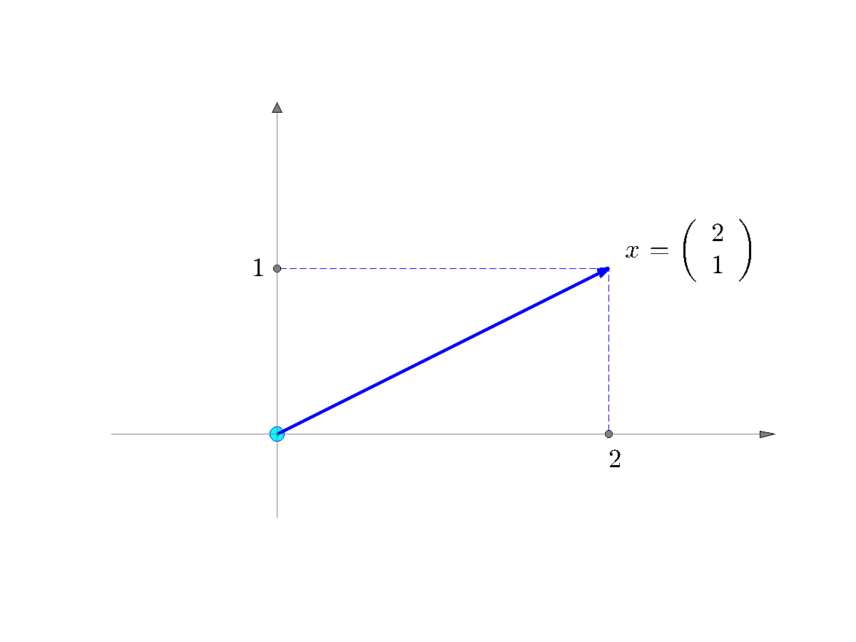 |
A vector can also represent a point in a multi-dimensional space , where each component corresponds to a coordinate of the point.
Example: The vector |
 in
in  .
.Examples:
Transpose
If is a column vector,  denotes the corresponding row vector, and vice-versa. Hence, if is the column vector above:

Sometimes we use the looser, in-line notation  , to denote a row or column vector, the orientation being understood from context.
Matlab syntax
A column vector  and its transpose
  can be declared in Matlab’s workspace as follows. Here, no room for loose notation: we use a semicolon to separate the components of a column vector, while we use commas for row vectors.
>> x = [2; 3.1; -4]; % declare a column vector using ";".
>> y = x'; % the prime operator ' transposes the vector.
>> y = [2,3.1,-4]; % can also declare a row vector with commas.
>> x(2) % this produces the second component of x.
>> x([1,3]) % this produces the 2-vector with the first and the third component of x.
Independence
A set of vectors  in
in  ,
,  . is said to be independent if and only if the following condition on a vector
  :
:

implies  . This means that no vector in the set can be expressed as a linear combination of the others.
Example: the vectors ![x^1 = [1, 2, 3]](https://ecampusontario.pressbooks.pub/app/uploads/quicklatex/quicklatex.com-14a8a64876015aff83cce4a0fcd55bcf_l3.png "Rendered by QuickLaTeX.com") and
and ![x^2 = [3, 6, 9]](https://ecampusontario.pressbooks.pub/app/uploads/quicklatex/quicklatex.com-c2f205d486729784946dc082a0430b33_l3.png "Rendered by QuickLaTeX.com") are not independent, since
are not independent, since  .
.
Subspace, span, affine sets
A subspace of is a subset that is closed under addition and scalar multiplication. Geometrically, subspaces are ‘‘flat’’ (like a line or plane in 3D) and pass through the origin.
An important result of linear algebra, which we will prove later, says that a subspace  can always be represented as the span of a set of vectors
  , , that is, as a set of the form

An affine set is a translation of a subspace — it is ‘‘flat’’ but does not necessarily pass through  , as a subspace would. (Think for example of a line, or a plane, that does not go through the origin.) So an affine set
  can always be represented as the translation of the subspace spanned by some vectors:

for some vectors  . In shorthand notation, we write
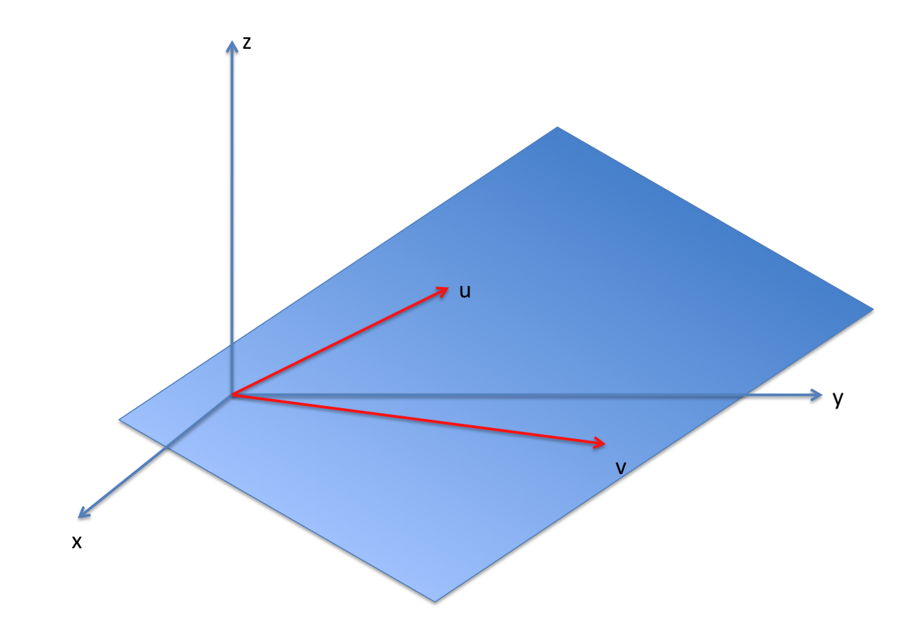 |
Example: In  , the span of the two vectors , the span of the two vectors
(2) [latex],\begin{align} v &= \begin{bmatrix} 1 \\ 3 \\ 0.1 \end{bmatrix} \end{align}[/latex] is the plane passing through the origin pictured in blue. |

When is the span of a single non-zero vector, the set is called a line passing through the point  . Thus, lines have the form
where  determines the direction of the line, and is a point through which it passes.
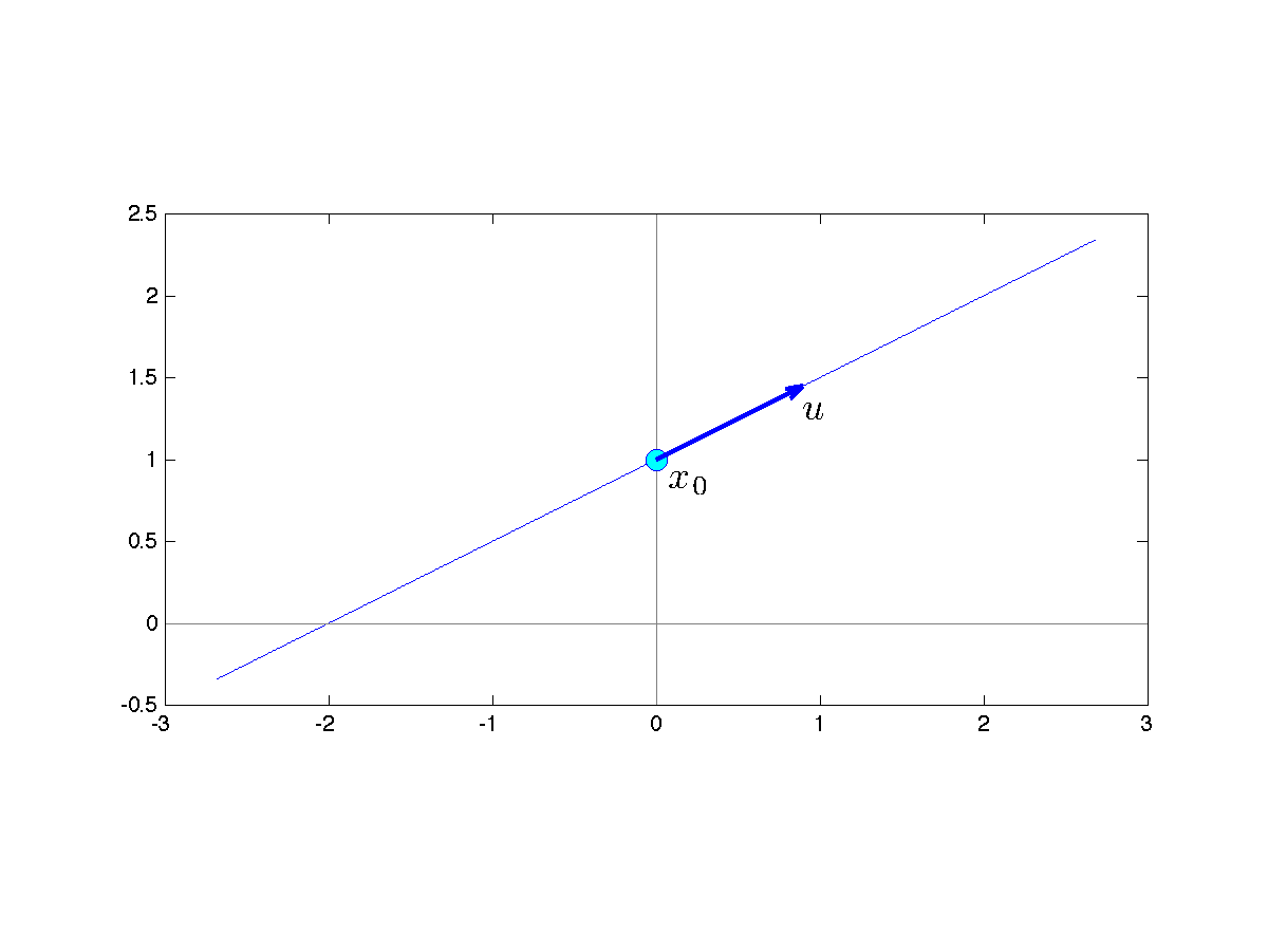 |
Example: A line in  passing through the point passing through the point  , with direction , with direction  . . |
Basis, dimension
Basis in 
A basis of is a set of independent vectors. If the vectors  form a basis, we can express any vector as a linear combination of the
  ‘s:
‘s:

for appropriate numbers  .
.
The standard basis (alternatively, natural basis) in consists of the vectors  , where ‘s components are all zero, except the -th, which is equal to
  . In , we have
(3) 
[latex],\begin{align} e_2 &:= \begin{pmatrix} 0 \\ 1 \\ 0 \end{pmatrix} \end{align}[/latex]
(4) 
Example: A basis in .
Basis of a subspace
The basis of a given subspace  is any independent set of vectors whose span is . If the vectors
  form a basis of , we can express any vector as a linear combination of the ‘s:

 .
.The number of vectors in the basis is actually independent of the choice of the basis (for example, in you need two independent vectors to describe a plane containing the origin). This number is called the dimension of  . We can accordingly define the dimension of an affine subspace, as that of the linear subspace of which it is a translation.
Examples:
- The dimension of a line is , since a line is of the form
 for some non-zero vector
  .
. - Dimension of an affine subspace.