You might think that with the advanced telescopes and detectors astronomers have today, they could directly image planets around nearby stars (which we call exoplanets). This has proved extremely difficult, however, not only because the exoplanets are faint, but also because they are generally lost in the brilliant glare of the star they orbit. The detection techniques that work best are indirect: they observe the effects of the planet on the star it orbits, rather than seeing the planet itself.

The first technique that yielded many planet detections is very high-resolution stellar spectroscopy. The Doppler effect lets astronomers measure the star’s radial velocity: that is, the speed of the star, toward us or away from us, relative to the observer. If there is a massive planet in orbit around the star, the gravity of the planet causes the star to wobble, changing its radial velocity by a small but detectable amount. The distance of the star does not matter, as long as it is bright enough for us to take very high quality spectra.

Measurements of the variation in the star’s radial velocity as the planet goes around the star can tell us the mass and orbital period of the planet. If there are several planets present, their effects on the radial velocity can be disentangled, so the entire planetary system can be deciphered—as long as the planets are massive enough to produce a measureable Doppler effect. This detection technique is most sensitive to large planets orbiting close to the star, since these produce the greatest wobble in their stars. It has been used on large ground-based telescopes to detect hundreds of planets, including one around Proxima Centauri, the nearest star to the Sun.

The second indirect technique is based on the slight dimming of a star when one of its planets transits, or crosses over the face of the star, as seen from Earth. Astronomers do not see the planet, but only detect its presence from careful measurements of a change in the brightness of the star over long periods of time. If the slight dips in brightness repeat at regular intervals, we can determine the orbital period of the planet. From the amount of starlight obscured, we can measure the planet’s size.

While some transits have been measured from Earth, large-scale application of this transit technique requires a telescope in space, above the atmosphere and its distortions of the star images. It has been most successfully applied from the NASA Kepler space observatory, which was built for the sole purpose of “staring” for 5 years at a single part of the sky, continuously monitoring the light from more than 150,000 stars. The primary goal of Kepler was to determine the frequency of occurrence of exoplanets of different sizes around different classes of stars. Like the Doppler technique, the transit observations favour discovery of large planets and short-period orbits.

Recent detection of exoplanets using both the Doppler and transit techniques has been incredibly successful. Within two decades, we went from no knowledge of other planetary systems to a catalog of thousands of exoplanets. Most of the exoplanets found so far are more massive than or larger in size than Earth. It is not that Earth analogs do not exist. Rather, the shortage of small rocky planets is an observational bias: smaller planets are more difficult to detect.

Analyses of the data to correct for such biases or selection effects indicate that small planets (like the terrestrial planets in our system) are actually much more common than giant planets. Also relatively common are “super Earths,” planets with two to ten times the mass of our planet as shown in Figure 9.6. We don’t have any of these in our solar system, but nature seems to have no trouble making them elsewhere. Overall, the Kepler data suggest that approximately one quarter of stars have exoplanet systems, implying the existence of at least 50 billion planets in our Galaxy alone.  For up to date information you can visit https://exoplanets.nasa.gov/keplerscience/ .

Transiting Planets by Size

Let’s look more closely at the progress in the detection of exoplanets. Figure 9.7 shows the planets that were discovered each year by the two techniques we discussed. In the early years of exoplanet discovery, most of the planets were similar in mass to Jupiter. This is because, as mentioned above, the most massive planets were easiest to detect. In more recent years, planets smaller than Neptune and even close to the size of Earth have been detected.

Masses of Exoplanets Discovered by Year

We also know that many exoplanets are in multiplanet systems. This is one characteristic that our solar system shares with exosystems. Since large disks can give rise to more than one centre of condensation, it is not too surprising that multi-planet systems are a typical outcome of planet formation. Astronomers have tried to measure whether multiple planet systems all lie in the same plane using astrometry. This is a difficult measurement to make with current technology, but it is an important measurement that could help us understand the origin and evolution of planetary systems.

Many of the planetary systems discovered so far do not resemble our own solar system. Consequently, we have had to reassess some aspects of the “standard models” for the formation of planetary systems. Science sometimes works in this way, with new data contradicting our expectations. The press often talks about a scientist making experiments to “confirm” a theory. Indeed, it is comforting when new data support a hypothesis or theory and increase our confidence in an earlier result. But the most exciting and productive moments in science often come when new data don’t support existing theories, forcing scientists to rethink their position and develop new and deeper insights into the way nature works.

Nothing about the new planetary systems contradicts the basic idea that planets form from the aggregation (clumping) of material within circumstellar disks. However, the existence of “hot Jupiters”—planets of jovian mass that are closer to their stars than the orbit of Mercury—poses the biggest problem. As far as we know, a giant planet cannot be formed without the condensation of water ice, and water ice is not stable so close to the heat of a star. It seems likely that all the giant planets, “hot” or “normal,” formed at a distance of several astronomical units from the star, but we now see that they did not necessarily stay there. This discovery has led to a revision in our understanding of planet formation that now includes “planet migrations” within the protoplanetary disk, or later gravitational encounters between sibling planets that scatter one of the planets inward.

Many exoplanets have large orbital eccentricity (recall this means the orbits are not circular). High eccentricities were not expected for planets that form in a disk. This discovery provides further support for the scattering of planets when they interact gravitationally. When planets change each other’s motions, their orbits could become much more eccentric than the ones with which they began.

There are several suggestions for ways migration might have occurred. Most involve interactions between the giant planets and the remnant material in the circumstellar disk from which they formed. These interactions would have taken place when the system was very young, while material still remained in the disk. In such cases, the planet travels at a faster velocity than the gas and dust and feels a kind of “headwind” (or friction) that causes it to lose energy and spiral inward. It is still unclear how the spiraling planet stops before it plunges into the star. Our best guess is that this plunge into the star is the fate for many protoplanets; however, clearly some migrating planets can stop their inward motions and escape this destruction, since we find hot Jupiters in many mature planetary systems.

The best possible evidence for an earthlike planet elsewhere would be an image. After all, “seeing is believing” is a very human prejudice. But imaging a distant planet is a formidable challenge indeed. Suppose, for example, you were a great distance away and wished to detect reflected light from Earth. Earth intercepts and reflects less than one billionth of the Sun’s radiation, so its apparent brightness in visible light is less than one billionth that of the Sun. Compounding the challenge of detecting such a faint speck of light, the planet is swamped by the blaze of radiation from its parent star.

Even today, the best telescope mirrors’ optics have slight imperfections that prevent the star’s light from coming into focus in a completely sharp point.

Direct imaging works best for young gas giant planets that emit infrared light and reside at large separations from their host stars. Young giant planets emit more infrared light because they have more internal energy, stored from the process of planet formation. Even then, clever techniques must be employed to subtract out the light from the host star. In 2008, three such young planets were discovered orbiting HR 8799, a star in the constellation of Pegasus, shown in Figure 9.8. Two years later, a fourth planet was detected closer to the star. Additional planets may reside even closer to HR 8799, but if they exist, they are currently lost in the glare of the star.

Since then, a number of planets around other stars have been found using direct imaging. However, one challenge is to tell whether the objects we are seeing are indeed planets or if they are brown dwarfs (failed stars) in orbit around a star.

Exoplanets around HR 8799

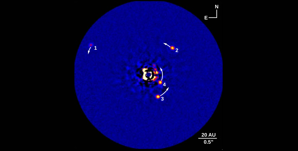
Direct imaging is an important technique for characterizing an exoplanet. The brightness of the planet can be measured at different wavelengths. These observations provide an estimate for the temperature of the planet’s atmosphere; in the case of HR 8799 planet 1, the colour suggests the presence of thick clouds. Spectra can also be obtained from the faint light to analyze the atmospheric constituents. A spectrum of HR 8799 planet 1 indicates a hydrogen-rich atmosphere, while the closer planet 4 shows evidence for methane in the atmosphere.

Another way to overcome the blurring effect of Earth’s atmosphere is to observe from space. Infrared may be the optimal wavelength range in which to observe because planets get brighter in the infrared while stars like our Sun get fainter, thereby making it easier to detect a planet against the glare of its star. Special optical techniques can be used to suppress the light from the central star and make it easier to see the planet itself. However, even if we go into space, it will be difficult to obtain images of Earth-size planets.

Before the discovery of exoplanets, most astronomers expected that other planetary systems would be much like our own—planets following roughly circular orbits, with the most massive planets several AU from their parent star. Such systems do exist in large numbers, but many exoplanets and planetary systems are very different from those in our solar system. Another surprise is the existence of whole classes of exoplanets that we simply don’t have in our solar system: planets with masses between the mass of Earth and Neptune, and planets that are several times more massive than Jupiter.

Kepler Results

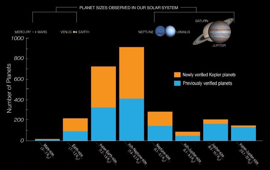
The Kepler telescope has been responsible for the discovery of most exoplanets, especially at smaller sizes, as illustrated in Figure 9.9, where the Kepler discoveries are plotted in yellow. You can see the wide range of sizes, including planets substantially larger than Jupiter and smaller than Earth. The absence of Kepler-discovered exoplanets with orbital periods longer than a few hundred days is a consequence of the 4-year lifetime of the mission. (Remember that three evenly spaced transits must be observed to register a discovery.) At the smaller sizes, the absence of planets much smaller than one earth radius is due to the difficulty of detecting transits by very small planets. In effect, the “discovery space” for Kepler was limited to planets with orbital periods less than 400 days and sizes larger than Mars.

Exoplanet Discoveries through 2015

One of the primary objectives of the Kepler mission was to find out how many stars hosted planets and especially to estimate the frequency of earthlike planets. Although Kepler looked at only a very tiny fraction of the stars in the Galaxy, the sample size was large enough to draw some interesting conclusions. While the observations apply only to the stars observed by Kepler, those stars are reasonably representative, and so astronomers can extrapolate to the entire Galaxy.

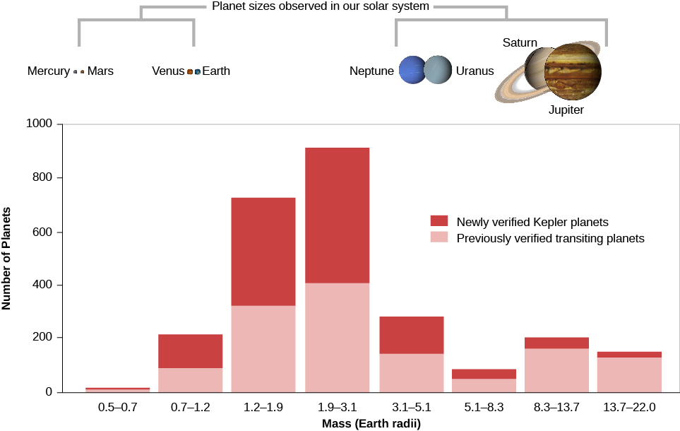
Figure 9.10 shows that the Kepler discoveries include many rocky, Earth-size planets, far more than Jupiter-size gas planets. This immediately tells us that the initial Doppler discovery of many hot Jupiters was a biased sample, in effect, finding the odd planetary systems because they were the easiest to detect. However, there is one huge difference between this observed size distribution and that of planets in our solar system. The most common planets have radii between 1.4 and 2.8 that of Earth, sizes for which we have no examples in the solar system. These have been nicknamed super-Earths, while the other large group with sizes between 2.8 and 4 that of Earth are often called mini-Neptunes.

Kepler Discoveries

What a remarkable discovery it is that the most common types of planets in the Galaxy are completely absent from our solar system and were unknown until Kepler’s survey. However, recall that really small planets were difficult for the Kepler instruments to find. So, to estimate the frequency of Earth-size exoplanets, we need to correct for this sampling bias. The result is the corrected size distribution shown in Figure 9.11. Notice that in this graph, we have also taken the step of showing not the number of Kepler detections but the average number of planets per star for solar-type stars (spectral types F, G, and K).

Size Distribution of Planets for Stars Similar to the Sun

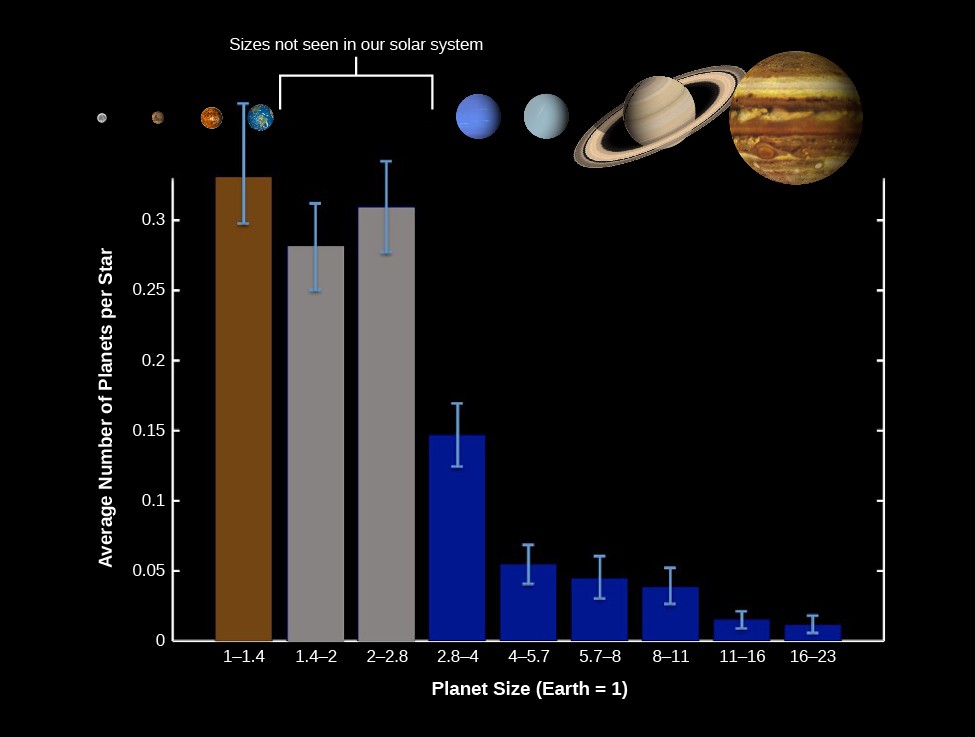
We see that the most common planet sizes of are those with radii from 1 to 3 times that of Earth—what we have called “Earths” and “super-Earths.” Each group occurs in about one-third to one-quarter of stars. In other words, if we group these sizes together, we can conclude there is nearly one such planet per star! And remember, this census includes primarily planets with orbital periods less than 2 years. We do not yet know how many undiscovered planets might exist at larger distances from their star.

To estimate the number of Earth-size planets in our Galaxy, we need to remember that there are approximately 100 billion stars of spectral types F, G, and K. Therefore, we estimate that there are about 30 billion Earth-size planets in our Galaxy. If we include the super-Earths too, then there could be one hundred billion in the whole Galaxy. This idea—that planets of roughly Earth’s size are so numerous—is surely one of the most important discoveries of modern astronomy.

Attribution

“14.4 Comparison with Other Planetary Systems – Exoplanets“, “21.4 Planets beyond the Solar System: Search and Discovery“, and  “21.5 Exoplanets Everywhere: What We Are Learning” from Douglas College Astronomy 1105 by Douglas College Department of Physics and Astronomy, are licensed under a Creative Commons Attribution 4.0 International License, except where otherwise noted. Adapted from Astronomy 2e.