7.3 Atmospheres of the Giant Planets
The atmospheres of the jovian planets are the parts we can observe or measure directly. Since these planets have no solid surfaces, their atmospheres are more representative of their general compositions than is the case with the terrestrial planets. These atmospheres also present us with some of the most dramatic examples of weather patterns in the solar system. As we will see, storms on these planets can grow bigger than the entire planet Earth.
Atmospheric Composition
When sunlight reflects from the atmospheres of the giant planets, the atmospheric gases leave their “fingerprints” in the spectrum of light. Spectroscopic observations of the jovian planets began in the nineteenth century, but for a long time, astronomers were not able to interpret the spectra they observed. As late as the 1930s, the most prominent features photographed in these spectra remained unidentified. Then better spectra revealed the presence of molecules of methane (CH4) and ammonia (NH3) in the atmospheres of Jupiter and Saturn.
At first astronomers thought that methane and ammonia might be the main constituents of these atmospheres, but now we know that hydrogen and helium are actually the dominant gases. The confusion arose because neither hydrogen nor helium possesses easily detected spectral features in the visible spectrum. It was not until the Voyager spacecraft measured the far-infrared spectra of Jupiter and Saturn that a reliable abundance for the elusive helium could be found.
The compositions of the two atmospheres are generally similar, except that on Saturn there is less helium as the result of the precipitation of helium that contributes to Saturn’s internal energy source. The most precise measurements of composition were made on Jupiter by the Galileo entry probe in 1995; as a result, we know the abundances of some elements in the jovian atmosphere even better than we know those in the Sun.
Voyagers in Astronomy
James Van Allen: Several Planets under His Belt
The career of physicist James Van Allen spanned the birth and growth of the space age, and he played a major role in its development. Born in Iowa in 1914, Van Allen received his PhD from the University of Iowa. He then worked for several research institutions and served in the Navy during World War II.
After the war, Van Allen (Figure 7.8) was appointed Professor of Physics at the University of Iowa. He and his collaborators began using rockets to explore cosmic radiation in Earth’s outer atmosphere. To reach extremely high altitudes, Van Allen designed a technique in which a balloon lifts and then launches a small rocket (the rocket is nicknamed “the rockoon”).
James Van Allen (1914–2006)
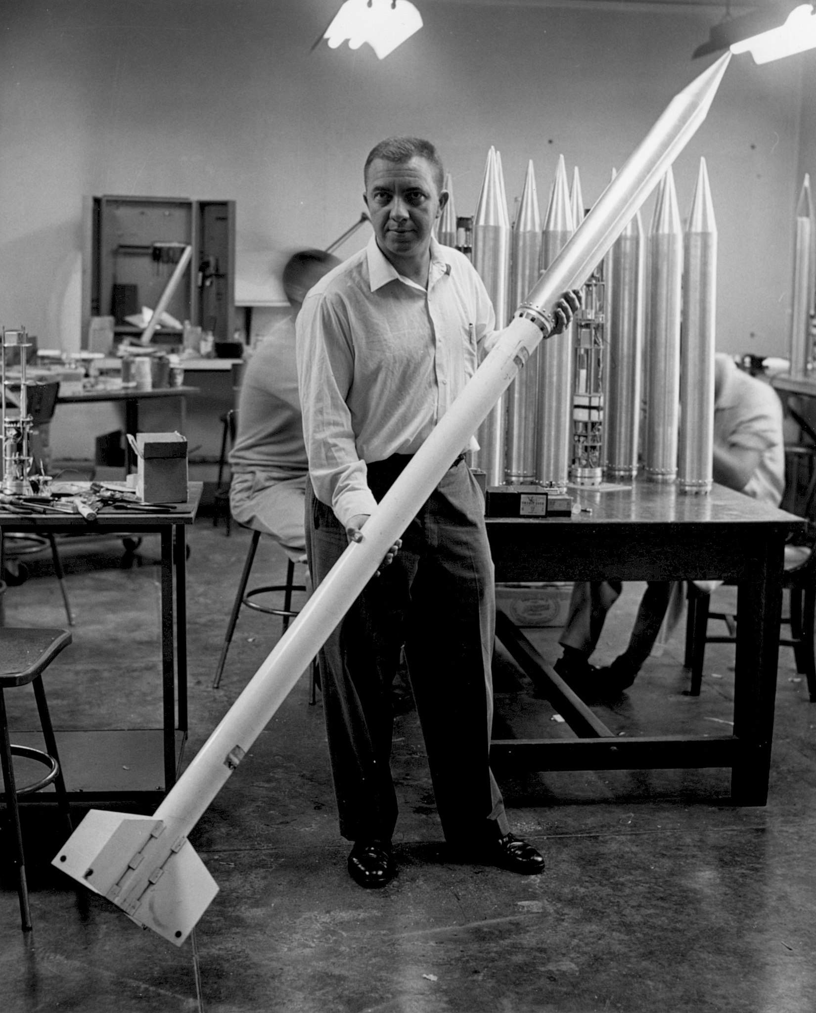
1955. James Van Allen holding a Loki rockoon in an Iowa fabrication lab courtesy of University of Iowa James A. Van Allen Collection
Over dinner one night in 1950, Van Allen and several colleagues came up with the idea of the International Geophysical Year (IGY), an opportunity for scientists around the world to coordinate their investigations of the physics of Earth, especially research done at high altitudes. In 1955, the United States and the Soviet Union each committed themselves to launching an Earth-orbiting satellite during IGY, a competition that began what came to be known as the space race. The IGY (stretched to 18 months) took place between July 1957 and December 1958.
The Soviet Union won the first lap of the race by launching Sputnik 1 in October 1957. The US government spurred its scientists and engineers to even greater efforts to get something into space to maintain the country’s prestige. However, the primary US satellite program, Vanguard, ran into difficulties: each of its early launches crashed or exploded. Simultaneously, a second team of rocket engineers and scientists had quietly been working on a military launch vehicle called Jupiter-C. Van Allen spearheaded the design of the instruments aboard a small satellite that this vehicle would carry. On January 31, 1958, Van Allen’s Explorer 1 became the first US satellite in space.
Unlike Sputnik, Explorer 1 was equipped to make scientific measurements of high-energy charged particles above the atmosphere. Van Allen and his team discovered a belt of highly charged particles surrounding Earth, and these belts now bear his name. This first scientific discovery of the space program made Van Allen’s name known around the world.
Van Allen and his colleagues continued to measure the magnetic and particle environment around planets with increasingly sophisticated spacecraft, including Pioneers 10 and 11, which made exploratory surveys of the environments of Jupiter and Saturn. Some scientists refer to the charged-particle zones around those planets as Van Allen belts as well. (Once, when Van Allen was giving a lecture at the University of Arizona, the graduate students in planetary science asked him if he would leave his belt at the school. It is now proudly displayed as the university’s “Van Allen belt.”)
Van Allen was a strong supporter of space science and an eloquent senior spokesperson for the American scientific community, warning NASA not to put all its efforts into human spaceflight, but to also use robotic spacecraft as productive tools for space exploration.
Clouds and Atmospheric Structure
The clouds of Jupiter (Figure 7.9) are among the most spectacular sights in the solar system, much beloved by makers of science-fiction films. They range in colour from white to orange to red to brown, swirling and twisting in a constantly changing kaleidoscope of patterns. Saturn shows similar but much more subdued cloud activity; instead of vivid colours, its clouds have a nearly uniform butterscotch hue (Figure 7.12).
Jupiter’s Colourful Clouds
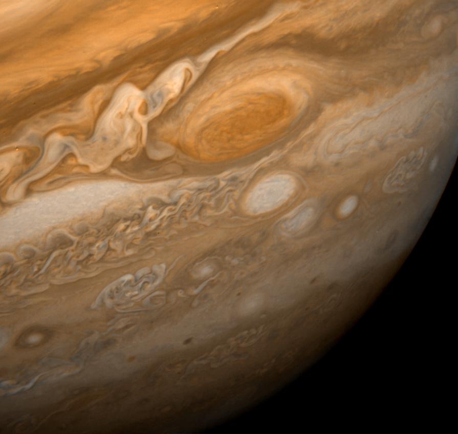
PIA00014: Jupiter Great Red Spot by NASA/JPL, NASA Media Licence.
Different gases freeze at different temperatures. At the temperatures and pressures of the upper atmospheres of Jupiter and Saturn, methane remains a gas, but ammonia can condense and freeze. (Similarly, water vapor condenses high in Earth’s atmosphere to produce clouds of ice crystals.) The primary clouds that we see around these planets, whether from a spacecraft or through a telescope, are composed of frozen ammonia crystals. The ammonia clouds mark the upper edge of the planets’ tropospheres; above that is the stratosphere, the coldest part of the atmosphere.
Saturn over Five Years

Saturn from 1996 to 2000 by NASA/Hubble, NASA Hubble Media Licence.
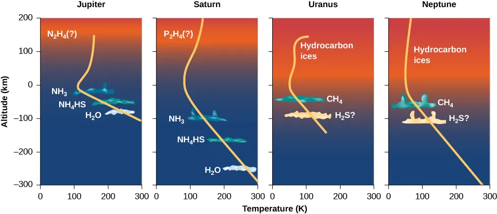
The diagrams in Figure 7.11 show the structure and clouds in the atmospheres of all four jovian planets. On both Jupiter and Saturn, the temperature near the cloud tops is about 140 K (only a little cooler than the polar caps of Mars). On Jupiter, this cloud level is at a pressure of about 0.1 bar (one tenth the atmospheric pressure at the surface of Earth), but on Saturn it occurs lower in the atmosphere, at about 1 bar. Because the ammonia clouds lie so much deeper on Saturn, they are more difficult to see, and the overall appearance of the planet is much blander than is Jupiter’s appearance.
Atmospheric Structure of the Jovian Planets
Within the tropospheres of these planets, the temperature and pressure both increase with depth. Through breaks in the ammonia clouds, we can see tantalizing glimpses of other cloud layers that can form in these deeper regions of the atmosphere—regions that were sampled directly for Jupiter by the Galileo probe that fell into the planet.
As it descended to a pressure of 5 bars, the probe should have passed into a region of frozen water clouds, then below that into clouds of liquid water droplets, perhaps similar to the common clouds of the terrestrial troposphere. At least this is what scientists expected. But the probe saw no water clouds, and it measured a surprisingly low abundance of water vapor in the atmosphere. It soon became clear to the Galileo scientists that the probe happened to descend through an unusually dry, cloud-free region of the atmosphere—a giant downdraft of cool, dry gas. Andrew Ingersoll of Caltech, a member of the Galileo team, called this entry site the “desert” of Jupiter. It’s a pity that the probe did not enter a more representative region, but that’s the luck of the cosmic draw. The probe continued to make measurements to a pressure of 22 bars but found no other cloud layers before its instruments stopped working. It also detected lightning storms, but only at great distances, further suggesting that the probe itself was in a region of clear weather.
Above the visible ammonia clouds in Jupiter’s atmosphere, we find the clear stratosphere, which reaches a minimum temperature near 120 K. At still higher altitudes, temperatures rise again, just as they do in the upper atmosphere of Earth, because here the molecules absorb ultraviolet light from the Sun. The cloud colours are due to impurities, the product of chemical reactions among the atmospheric gases in a process we call photochemistry. In Jupiter’s upper atmosphere, photochemical reactions create a variety of fairly complex compounds of hydrogen and carbon that form a thin layer of smog far above the visible clouds. We show this smog as a fuzzy orange region in Figure 7.11; however, this thin layer does not block our view of the clouds beneath it.
The visible atmosphere of Saturn is composed of approximately 75% hydrogen and 25% helium, with trace amounts of methane, ethane, propane, and other hydrocarbons. The overall structure is similar to that of Jupiter. Temperatures are somewhat colder, however, and the atmosphere is more extended due to Saturn’s lower surface gravity. Thus, the layers are stretched out over a longer distance, as you can see in Figure 7.11. Overall, though, the same atmospheric regions, condensation cloud, and photochemical reactions that we see on Jupiter should be present on Saturn (Figure 7.12).
Cloud Structure on Saturn

Strong Jet in False Colours by NASA/JPL-Caltech/Space Science Institute, NASA JPL Media Licence.
Saturn has one anomalous cloud structure that has mystified scientists: a hexagonal wave pattern around the north pole, shown in Figure 7.13. The six sides of the hexagon are each longer than the diameter of Earth. Winds are also extremely high on Saturn, with speeds of up to 1800 kilometres per hour measured near the equator.
Hexagon Pattern on Saturn’s North Pole
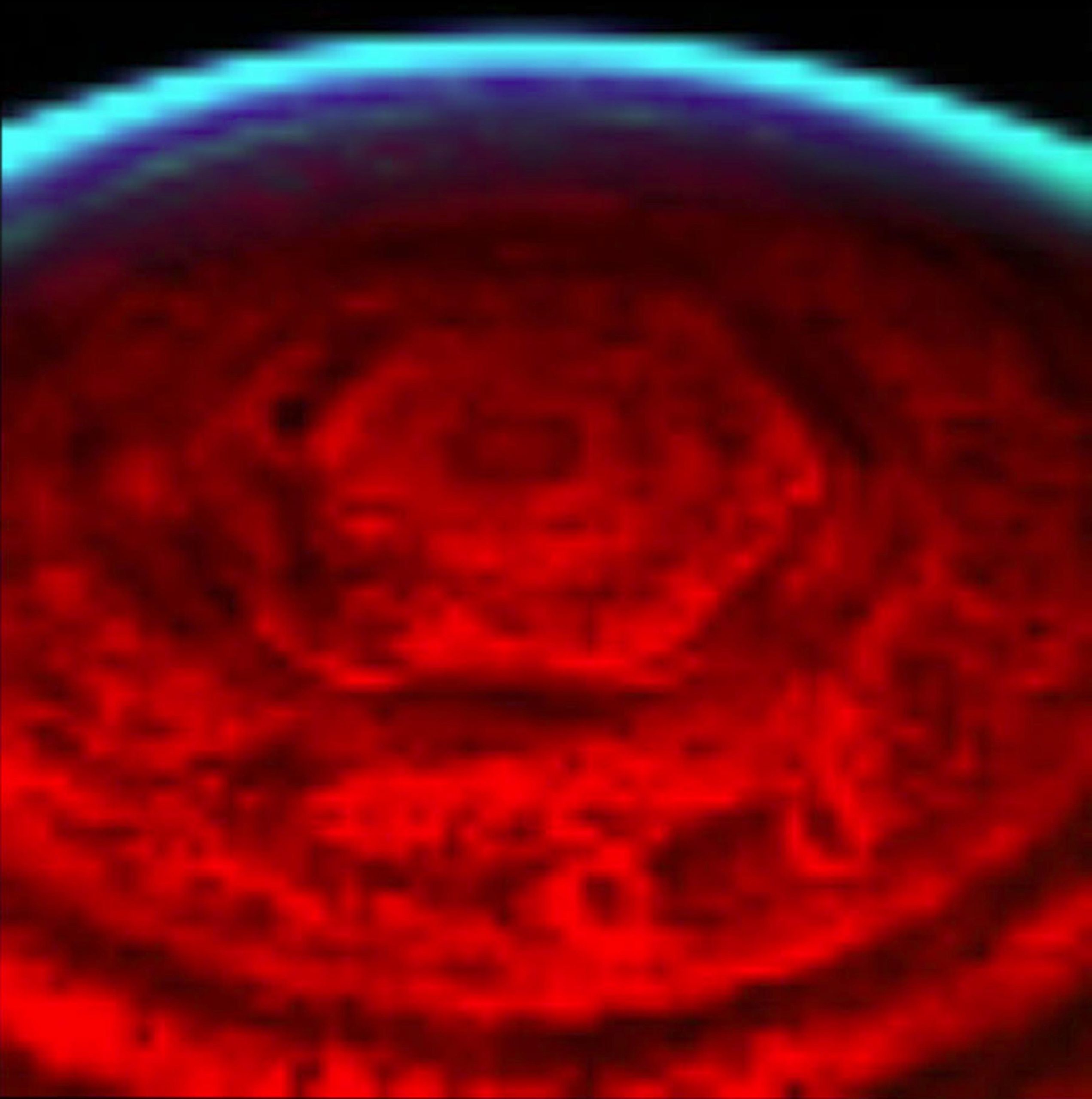
PIA09186: Saturn’s Strange Hexagon by NASA/JPL/University of Arizona, NASA Media Licence.
See images of Saturn’s hexagon with exaggerated colour in this brief NASA video.
Unlike Jupiter and Saturn, Uranus is almost entirely featureless as seen at wavelengths that range from the ultraviolet to the infrared. Calculations indicate that the basic atmospheric structure of Uranus should resemble that of Jupiter and Saturn, although its upper clouds (at the 1-bar pressure level) are composed of methane rather than ammonia. However, the absence of an internal heat source suppresses up-and-down movement and leads to a very stable atmosphere with little visible structure.
Neptune differs from Uranus in its appearance, although their basic atmospheric temperatures are similar. The upper clouds are composed of methane, which forms a thin cloud layer near the top of the troposphere at a temperature of 70 K and a pressure of 1.5 bars. Most the atmosphere above this level is clear and transparent, with less haze than is found on Uranus. The scattering of sunlight by gas molecules lends Neptune a pale blue colour similar to that of Earth’s atmosphere (Figure 7.14). Another cloud layer, perhaps composed of hydrogen sulfide ice particles, exists below the methane clouds at a pressure of 3 bars.
Neptune

Neptune Full Disk View by NASA/JPL, NASA JPL Media Licence.
Unlike Uranus, Neptune has an atmosphere in which convection currents—vertical drafts of gas—emanate from the interior, powered by the planet’s internal heat source. These currents carry warm gas above the 1.5-bar cloud level, forming additional clouds at elevations about 75 kilometres higher. These high-altitude clouds form bright white patterns against the blue planet beneath. Voyager photographed distinct shadows on the methane cloud tops, permitting the altitudes of the high clouds to be calculated. Figure 7.15 is a remarkable close-up of Neptune’s outer layers that could never have been obtained from Earth.
High Clouds in the Atmosphere of Neptune
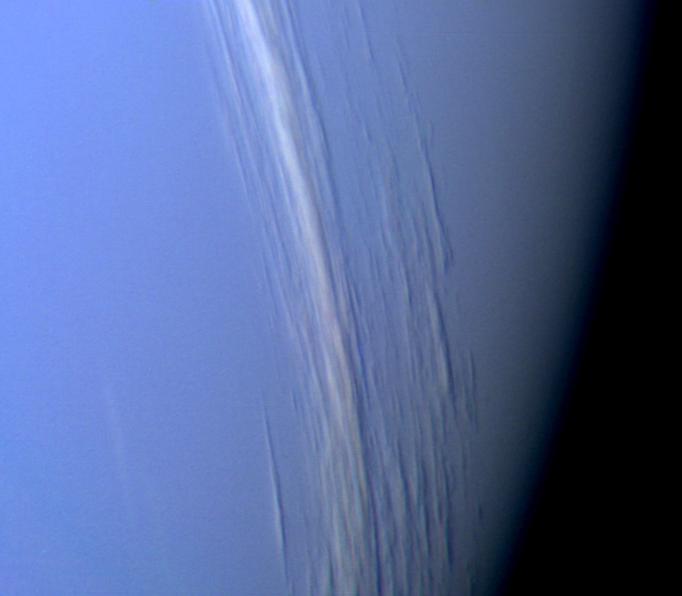
PIA00058: Neptune Clouds Showing Vertical Relief by NASA/JPL, NASA Media Licence.
Giant Storms on Giant Planets
The largest and most famous of Jupiter’s storms is the Great Red Spot, a reddish oval in the southern hemisphere that changes slowly; it was 25,000 kilometres long when Voyager arrived in 1979, but it had shrunk to 20,000 kilometres by the end of the Galileo mission in 2000 (Figure 7.17). The giant storm has persisted in Jupiter’s atmosphere ever since astronomers were first able to observe it after the invention of the telescope, more than 300 years ago. However, it has continued to shrink and has become more nearly circular, raising speculation that we may see its end within a few decades. Measurements from the Juno spacecraft of variations in Jupiter’s gravity field indicate that the depth of the Red Spot storm system is only a few hundred kilometres—a finding that challenges some of the models astronomers have made of this long-lasting weather system.
Storms on Jupiter
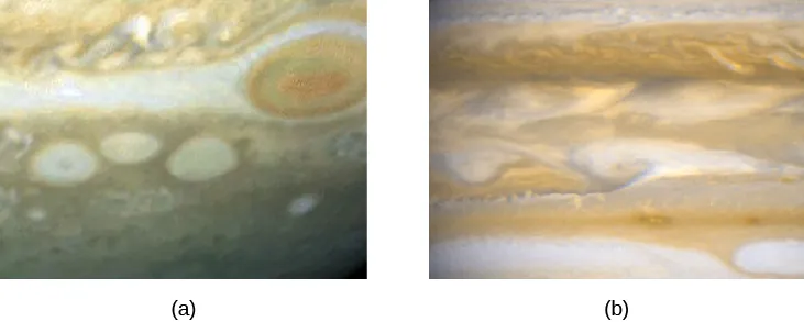
(a): PIA01262: Hubble Tracks Jupiter Storms by NASA/ New Mexico State Univ., NASA Media Licence.
(b): Jupiter – March 25, 2007 (Full Field) by NASA, ESA and A. Simon-Miller (NASA Goddard Space Flight Center), NASA Hubble Media Licence.
Jupiter’s Great Red Spot
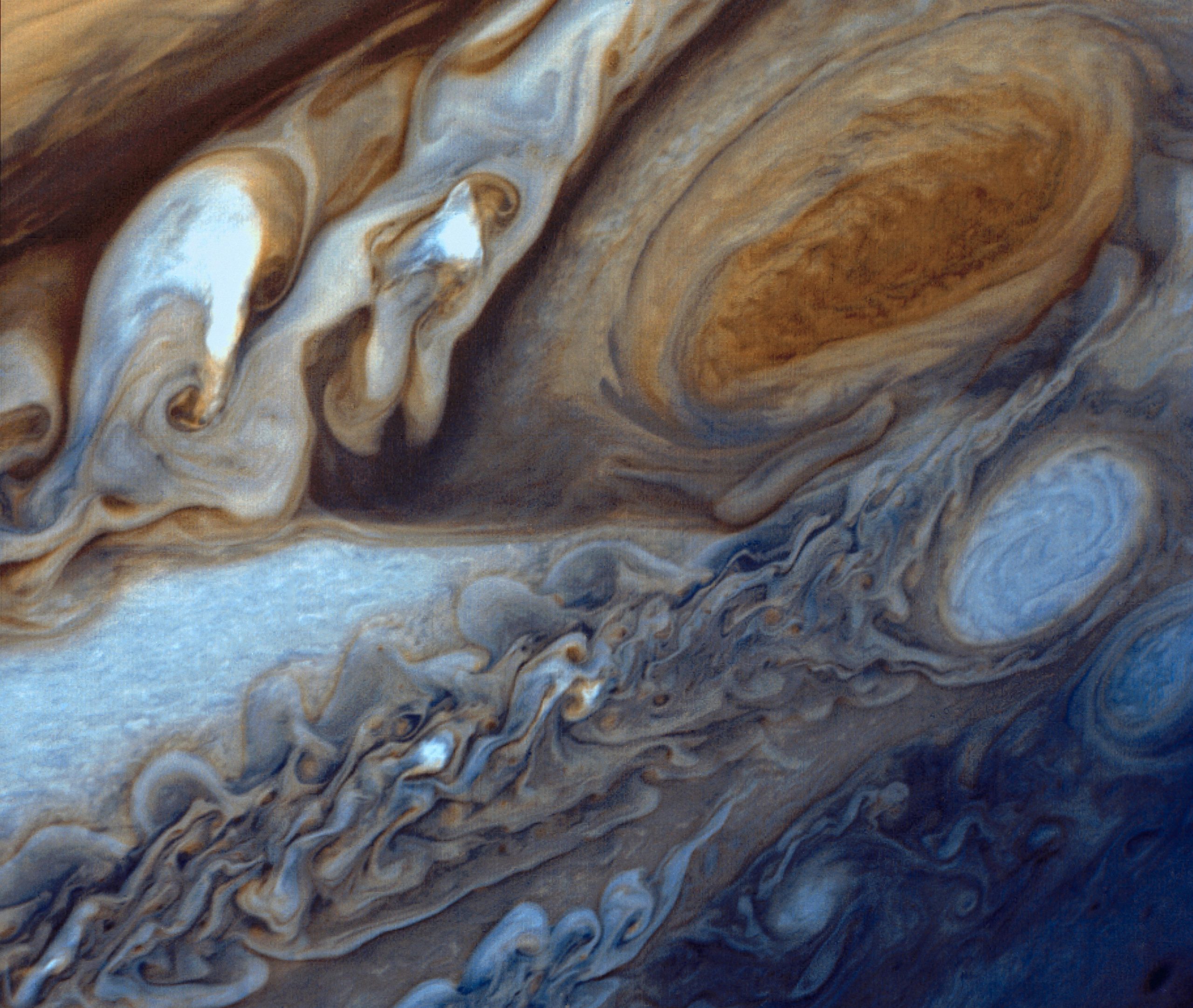
PIA01384: Jupiter’s Great Red Spot by NASA/JPL, NASA Media Licence.
In addition to its longevity, the Red Spot differs from terrestrial storms in being a high-pressure region; on our planet, such storms are regions of lower pressure. The Red Spot’s counterclockwise rotation has a period of six days. Three similar but smaller disturbances (about as big as Earth) formed on Jupiter in the 1930s. They look like white ovals, and one can be seen clearly below and to the right of the Great Red Spot in Figure 7.17. In 1998, the Galileo spacecraft watched as two of these ovals collided and merged into one.
We don’t know what causes the Great Red Spot or the white ovals, but we do have an idea how they can last so long once they form. On Earth, the lifetime of a large oceanic hurricane or typhoon is typically a few weeks, or even less when it moves over the continents and encounters friction with the land. Jupiter has no solid surface to slow down an atmospheric disturbance; furthermore, the sheer size of the disturbances lends them stability. We can calculate that on a planet with no solid surface, the lifetime of anything as large as the Red Spot should be measured in centuries, while lifetimes for the white ovals should be measured in decades, which is pretty much what we have observed.
Despite Neptune’s smaller size and different cloud composition, Voyager showed that it had an atmospheric feature surprisingly similar to Jupiter’s Great Red Spot. Neptune’s Great Dark Spot was nearly 10,000 kilometres long. On both planets, the giant storms formed at latitude 20° S, had the same shape, and took up about the same fraction of the planet’s diameter. The Great Dark Spot rotated with a period of 17 days, versus about 6 days for the Great Red Spot. When the Hubble Space Telescope examined Neptune in the mid-1990s, however, astronomers could find no trace of the Great Dark Spot on their images.
Although many of the details of the weather on the jovian planets are not yet understood, it is clear that if you are a fan of dramatic weather, these worlds are the place to look. We study the features in these atmospheres not only for what they have to teach us about conditions in the jovian planets, but also because we hope they can help us understand the weather on Earth just a bit better.
Example 7.1
Storms and Winds
The wind speeds in circular storm systems can be formidable on both Earth and the giant planets. Think about our big terrestrial hurricanes. If you watch their behavior in satellite images shown on weather outlets, you will see that they require about one day to rotate. If a storm has a diameter of [latex]400\;\text{km}[/latex] and rotates once in [latex]24\;\text{h}[/latex], what is the wind speed?
Solution
Speed equals distance divided by time. The distance in this case is the circumference ([latex]2\pi R[/latex] or [latex]\pi d[/latex]), or approximately [latex]1250\;\text{km}[/latex], and the time is [latex]24\;\text{h}[/latex], so the speed at the edge of the storm would be about [latex]52\;\text{km/h}[/latex]. Toward the center of the storm, the wind speeds can be much higher.
Exercise 7.1
Jupiter’s Great Red Spot rotates in [latex]6\;\text{d}[/latex] and has a circumference equivalent to a circle with radius [latex]10,000\;\text{km}[/latex]. Calculate the wind speed at the outer edge of the spot.
Solution
For the Great Red Spot of Jupiter, the circumference ([latex]2\pi R[/latex]) is about [latex]63,000\;\text{km}[/latex]. [latex]\text{Six d}[/latex] equals [latex]144\;\text{h}[/latex], suggesting a speed of about [latex]436\;\text{km/h}[/latex]. This is much faster than wind speeds on Earth.
Footnotes
2 Recall from earlier chapters that convection is a process in which liquids, heated from underneath, have regions where hot material rises and cooler material descends. You can see convection at work if you heat oatmeal on a stovetop or watch miso soup boil.
Attribution
“11.3 Atmospheres of the Giant Planets” from Astronomy 2e by Andrew Fraknoi, David Morrison, Sidney C. Wolff, © OpenStax – Rice University is licensed under a Creative Commons Attribution 4.0 International License, except where otherwise noted.
