13.5 Quasars
The name “quasars” started out as short for “quasi-stellar radio sources” (here “quasi-stellar” means “sort of like stars”). The discovery of radio sources that appeared point-like, just like stars, came with the use of surplus World War II radar equipment in the 1950s. Although few astronomers would have predicted it, the sky turned out to be full of strong sources of radio waves. As they improved the images that their new radio telescopes could make, scientists discovered that some radio sources were in the same location as faint blue “stars.” No known type of star in our Galaxy emits such powerful radio radiation. What then were these “quasi-stellar radio sources”?
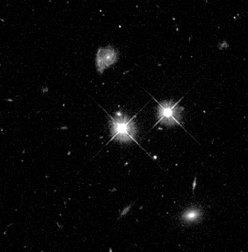
The answer came when astronomers obtained visible-light spectra of two of those faint “blue stars” that were strong sources of radio waves as shown in Figure 13.14. Spectra of these radio “stars” only deepened the mystery: they had emission lines, but astronomers at first could not identify them with any known substance. By the 1960s, astronomers had a century of experience in identifying elements and compounds in the spectra of stars. Elaborate tables had been published showing the lines that each element would produce under a wide range of conditions. A “star” with unidentifiable lines in the ordinary visible light spectrum had to be something completely new.
Typical Quasar

QSO H1821+643 Indicates a Universe Filled with Hydrogen by Todd M. Tripp (Princeton) et al. WIYN Observatory, NOAO, NSF; & HST, NASA, NASA Media License.
In 1963 at Caltech’s Palomar Observatory, Maarten Schmidt was puzzling over the spectrum of one of the radio stars, which was named 3C 273 because it was the 273rd entry in the third Cambridge catalog of radio sources (Figure 13.15). There were strong emission lines in the spectrum, and Schmidt recognized that they had the same spacing between them as the Balmer lines of hydrogen. But the lines in 3C 273 were shifted far to the red of the wavelengths at which the Balmer lines are normally located. Indeed, these lines were at such long wavelengths that if the redshifts were attributed to the Doppler effect, 3C 273 was receding from us at a speed of 45,000 kilometres per second, or about 15% the speed of light! Since stars don’t show Doppler shifts this large, no one had thought of considering high redshifts to be the cause of the strange spectra.
Quasar 3C 273

Best image of bright quasar 3C 273 by ESA/Hubble/NASA, ESA Standard License.
The puzzling emission lines in other star-like radio sources were then reexamined to see if they, too, might be well-known lines with large redshifts. This proved to be the case, but the other objects were found to be receding from us at even greater speeds. Their astounding speeds showed that the radio “stars” could not possibly be stars in our own Galaxy. Any true star moving at more than a few hundred kilometres per second would be able to overcome the gravitational pull of the Galaxy and completely escape from it. (As we shall see later in this chapter, astronomers eventually discovered that there was also more to these “stars” than just a point of light.)
It turns out that these high-velocity objects only look like stars because they are compact and very far away. Later, astronomers discovered objects with large redshifts that appear star-like but have no radio emission. Observations also showed that quasars were bright in the infrared and X-ray bands too, and not all these X-ray or infrared-bright quasars could be seen in either the radio or the visible-light bands of the spectrum. Today, all these objects are referred to as quasi-stellar objects (QSOs), or, as they are more popularly known, quasars. (The name was also soon appropriated by a manufacturer of home electronics.)
Over a million quasars have now been discovered, and spectra are available for over a hundred thousand. All these spectra show redshifts, none show blueshifts, and their redshifts can be very large. Yet in a photo they look just like stars as shown in Figure 13.16.
Typical Quasar Imaged by the Hubble Space Telescope
Hubble’s 100,000th Exposure by Charles Steidel (CIT)/NASA/ESA, ESA Standard License.
In the record-holding quasars, the first Lyman series line of hydrogen, with a laboratory wavelength of 121.5 nanometres in the ultraviolet portion of the spectrum, is shifted all the way through the visible region to the infrared. At such high redshifts, the simple formula for converting a Doppler shift to speed must be modified to take into account the effects of the theory of relativity. If we apply the relativistic form of the Doppler shift formula, we find that these redshifts correspond to velocities of about 96% of the speed of light.
Given their large distances, quasars have to be extremely luminous to be visible to us at all—far brighter than any normal galaxy. In visible light alone, most are far more energetic than the brightest elliptical galaxies. But, as we saw, quasars also emit energy at X-ray and ultraviolet wavelengths, and some are radio sources as well. When all their radiation is added together, some QSOs have total luminosities as large as a hundred trillion Suns (1014LSun), which is 10 to 100 times the brightness of luminous elliptical galaxies.
Finding a mechanism to produce the large amount of energy emitted by a quasar would be difficult under any circumstances. But there is an additional problem. When astronomers began monitoring quasars carefully, they found that some vary in luminosity on time scales of months, weeks, or even, in some cases, days. This variation is irregular and can change the brightness of a quasar by a few tens of percent in both its visible light and radio output.
Think about what such a change in luminosity means. A quasar at its dimmest is still more brilliant than any normal galaxy. Now imagine that the brightness increases by 30% in a few weeks. Whatever mechanism is responsible must be able to release new energy at rates that stagger our imaginations. The most dramatic changes in quasar brightness are equivalent to the energy released by 100,000 billion Suns. To produce this much energy we would have to convert the total mass of about ten Earths into energy every minute.
Moreover, because the fluctuations occur in such short times, the part of a quasar that is varying must be smaller than the distance light travels in the time it takes the variation to occur—typically a few months. To see why this must be so, let’s consider a cluster of stars 10 light-years in diameter at a very large distance from Earth (see Figure 13.17 in which Earth is off to the right). Suppose every star in this cluster somehow brightens simultaneously and remains bright. When the light from this event arrives at Earth, we would first see the brighter light from stars on the near side; 5 years later we would see increased light from stars at the center. Ten years would pass before we detected more light from stars on the far side.
How the Size of a Source Affects the Timescale of Its Variability
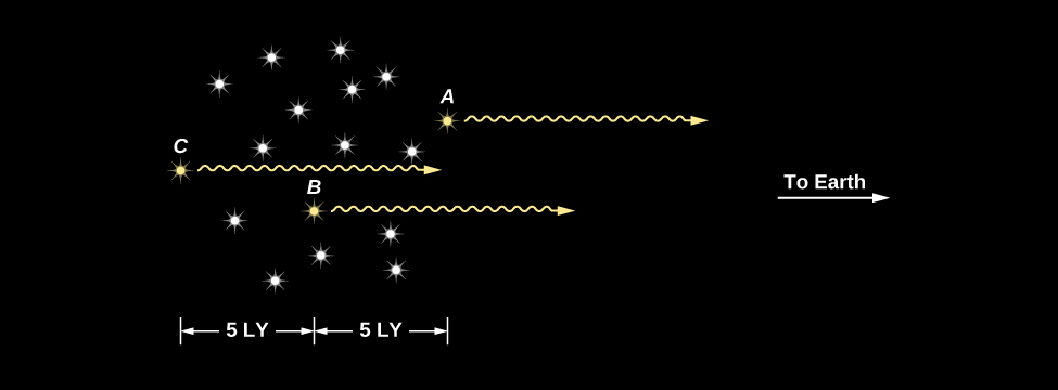
Even though all stars in the cluster brightened at the same time, the fact that the cluster is 10 light-years wide means that 10 years must elapse before the increased light from every part of the cluster reaches us. From Earth we would see the cluster get brighter and brighter, as light from more and more stars began to reach us. Not until 10 years after the brightening began would we see the cluster reach maximum brightness. In other words, if an extended object suddenly flares up, it will seem to brighten over a period of time equal to the time it takes light to travel across the object from its far side.
We can apply this idea to brightness changes in quasars to estimate their diametres. Because quasars typically vary (get brighter and dimmer) over periods of a few months, the region where the energy is generated can be no larger than a few light-months across. If it were larger, it would take longer than a few months for the light from the far side to reach us.
How large is a region of a few light-months? Pluto, usually the outermost (dwarf) planet in our solar system, is about 5.5 light-hours from us, while the nearest star is 4 light-years away. Clearly a region a few light months across is tiny relative to the size of the entire Galaxy. And some quasars vary even more rapidly, which means their energy is generated in an even smaller region. Whatever mechanism powers the quasars must be able to generate more energy than that produced by an entire galaxy in a volume of space that, in some cases, is not much larger than our solar system.
Even before the discovery of quasars, there had been hints that something very strange was going on in the centers of at least some galaxies. Back in 1918, American astronomer Heber Curtis used the large Lick Observatory telescope to photograph the galaxy Messier 87 in the constellation Virgo. On that photograph, he saw what we now call a jet coming from the centre, or nucleus, of the galaxy, pictured in Figure 13.18. This jet literally and figuratively pointed to some strange activity going on in that galaxy nucleus. But he had no idea what it was. No one else knew what to do with this space oddity either.
The random factoid that such a central jet existed lay around for a quarter century, until Carl Seyfert, a young astronomer at Mount Wilson Observatory, also in California, found half a dozen galaxies with extremely bright nuclei that were almost stellar, rather than fuzzy in appearance like most galaxy nuclei. Using spectroscopy, he found that these nuclei contain gas moving at up to two percent the speed of light. That may not sound like much, but it is 6 million miles per hour, and more than 10 times faster than the typical motions of stars in galaxies.
M87 Jet
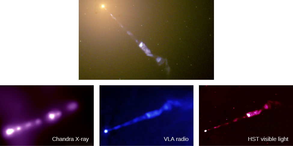
Credit top: M87 jet by NASA, The Hubble Heritage Team(STScI/AURA), NASA Media License.
Credit bottom: M87 Jet: Chandra Sheds Light on the Knotty Problem of the M87 Jet by X-ray: H. Marshall (MIT), et al., CXC, NASA; Radio: F. Zhou, F. Owen (NRAO), J. Biretta (STScI); Optical: E. Perlman (UMBC), et al., NASA Media License.
After decades of study, astronomers identified many other strange objects beyond our Milky Way Galaxy; they populate a whole “zoo” of what are now called active galaxies or active galactic nuclei (AGN). Astronomers first called them by many different names, depending on what sorts of observations discovered each category, but now we know that we are always looking at the same basic mechanism. What all these galaxies have in common is some activity in their nuclei that produces an enormous amount of energy in a very small volume of space. In the next section, we describe a model that explains all these galaxies with strong central activity—both the AGNs and the QSOs.
Attribution
“27.1 Quasars” from Douglas College Astronomy 1105 by Douglas College Department of Physics and Astronomy, is licensed under a Creative Commons Attribution 4.0 International License, except where otherwise noted. Adapted from Astronomy 2e.
