Lab 2 – Spatial Data Sources for GIS Projects
Introduction
Archives and Databases
In the previous lab, we discussed some different meanings of the term “archive”, and settled on a broad definition: that an archive is simply a collection of things. In a digital archive, these can be digital representations of objects, or they can be objects which have always been digital. By this definition, the sources of spatial data that we will consider in this lab could be called archives. However, not every person would consider them so! They could also be described as databases, since they are computerized structures which store data. You might prefer this term, since these data sources are intended more to distribute data than to preserve it, which many people would consider a key role of an archive. These terms will be used interchangeably in this lab, along with the term spatial data source.
Spatial Databases
Spatial data are available from a wide range of sources. Because this course focuses on the digital humanities, we will focus on digital spatial data. However, you should be aware that physical archives can also be rich sources of spatial data. Generally this will be in the form of maps, but other texts can be useful too; for example, an archaeological report that describes the location of excavations could be said to contain spatial data. Note that in order to use either of these theoretical physical data sources in modern mapping applications, they would need to be digitized. In the case of maps, this could involve scanning the map and then georeferencing it, while in the case of books and reports you might need to read the text and manually create spatial data points. Both of these processes will be covered in future labs. Equally, the contents of a digital archive could be printed, and made physical. Thus, the lines between physical and digital archives and data are more permeable than they may first appear!
Many of the archives discussed in this lab will be run by government institutions. There are many reasons that governments collect, and sometimes also disseminate, large amounts of spatial data. For one thing, governments need data in order to plan and allocate resources effectively. Data about crime rates could be used to plan police patrol routes, while data describing forest characteristics could be used to determine where forestry licenses will be available. There are several key points to note here. First, these activities are not neutral, and can be used to dispossess or disadvantage certain groups. Some scholars feel, for example, that using crime data collected based on structurally racist practices can only reinforce those practices, and worse, will make them seem scientific and acceptable, because they are supported by data (Jefferson, 2018). In another example, data collection about physical resources in a territory is necessary in order to control those resources (Peluso, 1995). However, the second important point about these data is that you do not have to use them in the way they were intended to be used. For example, the very datasets used to control resources can also be used to tell the story of that control. This can be a component of counter mapping, which aims to speak back to the power structures usually reinforced by maps and spatial data.
Another key consideration in understanding why so many accessible spatial archives and databases are government run is that spatial data tend to be expensive, especially if they are to be collected consistently over a large area or large span of time. Surveys, whether physical or cultural, require both people and equipment, all of which must be paid for and organized somehow. Governments are often ideally placed to do both of these things. Further, it is often in their interests to distribute the spatial data they have collected, so that their citizens can make use of it in various ways which may benefit the economy or advance the state of knowledge. This can also be true of other powerful institutions, such as universities or non-governmental organizations. As with government databases, it is important to consider why these databases are being made available to you, how they are funded, and what practices and agendas might have resulted in the data they contain. There is a tendency to assume that the bigger an institution is, the more trustworthy the data it produces is likely to be, but you should critically evaluate all your data sources.
In addition to governmental and institutional spatial databases, you may occasionally come across a community-based spatial database. One of the most famous is OpenStreetMap [https://www.openstreetmap.org/about], which is updated and maintained by users worldwide, based on their own local knowledge. From a critical evaluation perspective, this makes things even trickier, because every piece of data will have a different agenda and set of beliefs behind it, all working within the structure of the database itself. In the end, you will need to make judgement calls about the most appropriate data source for your own projects, based on your own concerns.
Critical Considerations for Maps and Mapping
The previous section outlined some of the major critical considerations for spatial databases. These are much the same as for any archive. However, you should be aware that maps deserve some particular attention in this regard. This is because of how powerful they are. You may have heard the saying that a picture is worth a thousand words; this can certainly be true of maps. They are able to communicate vast amounts of information quickly; sometimes at a glance. They can persuade, and can also shape the real world, since they are used as tools in political, corporate, and personal decision making. This is true both of the maps you read and the maps you make, and as with your spatial data sources, you should always critically assess the maps you work with. Further readings on this topic are available in Appendix 2.
How GIS Software Will be Used in these Labs
Since this course discusses the intersection between the spatial and digital humanities, the majority of the labs will ask you to work with digital spatial data files. Just like you need specific kinds of software to take full advantage of spreadsheets or PDF documents, you need a certain kind of software to work with spatial data. A software package for working with spatial data is often referred to as a GIS, which is short for geographic information system. There are many GIS packages available; while completing this course you will probably come across many examples of spatial storytelling using ArcGIS and StoryMaps, which are produced by the company ESRI. However, the labs will focus on QGIS, which is a free and open source GIS, with very similar functionality to paid GIS packages like ArcGIS.
You do not need any GIS experience to complete these labs. All of the operations you are asked to carry out are very basic, and described in detail. Important GIS concepts that you may or may not be familiar with, but which don’t have an immediate bearing on the outcome of the lab, are explained in the appendices. For information on how to install QGIS, as well as a quick guide to its basic functionality, see the tutorial provided with this course, or consult online sources.
Downloading Spatial Data Manually
As you learned in the previous lab, there are many archives available on the internet. Most will be specialized in some way, being based around a theme and often a particular type of data. This section will demonstrate how to download spatial data from several sites, mainly operated by government organizations.
While the files you will learn how to download in this lab are not explicitly historical, or in fact necessarily related to any of the humanities, they will still be useful in your mapping projects. In particular, they will allow you add context to your historical data by showing your readers how the data relate to modern geopolitical boundaries or other features they might recognize. You may also find other uses for them as you progress through the course.
GeoHub
GeoHub [https://geohub.lio.gov.on.ca/] is Ontario’s official geospatial data website. Many of the most common datasets, including shapefiles of features like provincial parks, roads, and waterbodies, are available for anyone to download. If you need a refresher on what a shapefile is, consult Appendix 1. Other datasets, such as high resolution aerial imagery, must be purchased.
- Use the link above to go the GeoHub home page.
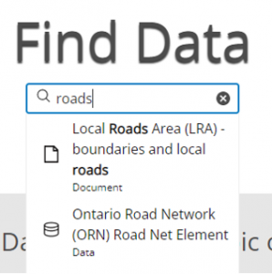
- If you know what you want to make a map of, try typing a keyword in the search bar.
- A list of relevant items will drop down from the search bar. Look for one labelled “data”, with an icon of three stacked disks next to it – this indicates a dataset, rather than a document describing a dataset. Click the desired item to access its page.
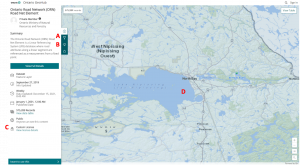
- For spatial datasets, the item page will look something like figure 2. Key components have been highlighted for you.
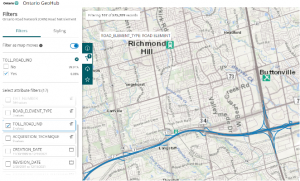
- If you wish to download only certain parts of the dataset, you can achieve this by using the filter button. Clicking this will bring up a list of attributes that you can filter the dataset by. For example, if you only wished the map toll roads, you would put a checkmark next to “TOLL_ROAD_IND”, and then a checkmark next to “Yes” at the top of the screen.
- To download your dataset, click the download button. This will provide you with a list of file formats, and options for downloading each one. We suggest using shapefiles, but any of the options except for CSV will also work.
- If you have applied filters to your dataset and only want to download the filtered items, turn on the “Toggle Filters” button before clicking download. However, you should be aware that the file must be generated from scratch, which is time consuming. If you don’t have time to wait, simply download the full file.
- If you find that the Shapefile will not download, try scrolling to the very bottom of the download pane, and clicking “Complete Shapefile” instead.
- The file will likely be stored in your downloads folder; save it with a name you will remember in a location you can find easily.
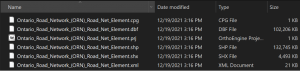
- Note that the shapefile is actually a collection of files, all with the same name but with different file extensions. These files must be stored together in order to work.
If you are simply exploring what GeoHub has to offer, and aren’t looking for any particular dataset, you can scroll down the home page to the “Browse Topics” section, and browse through lists of datasets organized by theme. Even further down the page are a list of online interactive maps that allow you to explore various themes, such as topographic information, recent forest fires, and river flow.
Having downloaded your data, you will probably want to view it in a GIS, to make sure it was actually what you wanted. Opening files in QGIS is very easy:
- Open QGIS, and choose a project from the list of templates provided to you.
- In the browser panel, navigate to the location where your file is stored.
- There may be several copies of your file with the same name, depending where you downloaded it from. Look for the one with the extension “.shp”.
- Drag this file from the browser panel into the main body of your map, or into the layers panel.

Statistics Canada
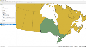
Sometimes, you might want to download the borders of one or more provinces, or even of a particular city. The best place to find boundary files of this type is the Statistics Canada website [https://www12.statcan.gc.ca/census-recensement/2011/geo/bound-limit/bound-limit-eng.cfm]. At present, boundary files are available going back to 2001; they are based on the boundaries used to organize census data, and thus can change slightly from one census to the next.
- Open the link above to reach the Boundary Files page of the Stats Can website.
- Choose your census year. The download process is the same regardless of the year.
- Specify your desired language and your output format. We will use the “ArcGIS” format, which is just a shapefile; these files are portable between many different GIS packages.
- Decide what boundary file you need for your particular purpose. Provinces/territories are an obvious choice if you are mapping all of Canada, or just want an outline of a single province. Census tracts are a good choice for mapping larger cities. Note that cartographic boundary files only show land areas, while the digital boundary files include areas of coastal waters that Canada considers to be part of its territory. Cartographic boundary files will be more recognizable to most map readers.
- Click “Continue” to move on to the next page. It will have a link to your requested file; simply click to download.
USGS Earth Explorer
So far, the instructions in this lab have shown you how to download shapefiles, which as you can see are more or less drawings of geographic features. However, it is also possible to download satellite imagery, which is a photograph of the earth’s surface rather than a drawing. There are numerous sites that allow you to download satellite imagery, and some sites allow you to choose between a number of satellite platforms. Generally speaking, coarser resolution imagery is likely to be freely available, while finer resolution imagery, in which more details are visible, costs money. We will use the United States Geological Survey website to download some imagery. Note that you do need an account to download this imagery, and that the site comes with a sizeable disclaimer indicating that use of the website is monitored by the US government; if for this or any other reason you would prefer not to create an account, feel free to skip this section.
- Log in to the EarthExplorer [https://earthexplorer.usgs.gov/] website.
- Using either the map, or the search box to the left of the screen, find the area you wish to map. If you are searching for a location outside of the US, you must click the “World Features” button above the search bar.
- Once you have found your study area, use the map to zoom in to approximately the boundaries of your area of interest. Then, in the second pane at the left of the screen, find and click the “Use Map” button. This defines the area you were zoomed in to as the area you wish to download imagery for.
- In the third pane, define the dates you are interested in. Then click the “Data Sets >>” button.
- This is where you can choose which satellite to download imagery from. Both Landsat and Sentinel 2 data are free to download; here we will use Sentinel because it has a finer spatial resolution, and thus is more detailed. Click the plus sign next to Sentinel, and place a checkmark next to the only available dataset.
- Click the “Additional Criteria >>” button. While these advanced settings are optional, it can be helpful to set “Cloud Cover” to a low value to ensure clouds are not covering your imagery.
- Click the “Results” button to see a list of available images meeting your search criteria.
- Each image will have a number of icons below it which allow you to preview and download it. It is particularly helpful to view a preview of your image on the map, because this will help you determine if there are clouds covering any area that you are interested in.
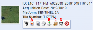
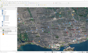
- When you have chosen an image, click the download button. A dialogue box will pop up prompting you to choose a format; download the JPEG2000 option. It may take a minute or two for the download to begin.
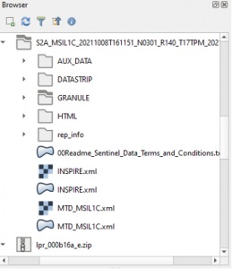
- Once you have downloaded your image, unzip it.
- As with a shapefile, your sentinel image is made up of many different files. It is best not to delete any of these, or your imagery may not open.
- To open your sentinel imagery in QGIS, look for the file labelled MTD_MSIL1C.xml, and drag this into the map pane. A dialogue box will open; make sure the row with layer ID 0 is highlighted, and then click OK. This will open a true colour image.
Using APIs
The previous sections of this lab have shown you how to download spatial data from several different sources. However, these techniques require you to use the website’s graphical interface. What if you would prefer to download data directly into the software package you are already using? This can be accomplished using APIs.
An API is an application programming interface, and allows two software packages, or in this case a software package and a website or database, to connect to one another. This allows you to download data without using the graphical interfaces you have used in the previous section of the lab. APIs have other uses, too – for example, you can embed Google Maps in your own website using an API.
In this example, we will create a connection to GeoHub, and rather than downloading the dataset, import it directly into QGIS. This method might be particularly useful if you lack storage space on your computer, but you should keep in mind that zooming and rendering may be slower, as the data is stored remotely.
Note that many other websites allow you to download data using APIs. Most will also allow you to download data manually. For example, ESRI’s Open Data Portal [https://hub.arcgis.com/search] collates datasets from many different sources. You may notice that this looks very similar to GeoHub, which is because GeoHub is built using ESRI technology. This is useful; if you can use GeoHub, you already know how to find and download data from ESRI’s portal.
- Navigate to GeoHub [https://geohub.lio.gov.on.ca/], and find a dataset of interest to you. Go to its item page.
- You could download your data using the download button; however, this time we will use an API, so you need to click the blue “I want to use this” button at the bottom of the page.
- Click the “View API Resources” button. There are several links provided. Both OCG WMS and GeoJSON work in QGIS, but GeoJSON is simpler to use, so copy this link.
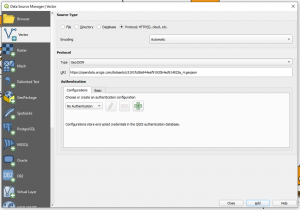
- Go to QGIS, and from the Layer menu at the top of the screen, choose “Add Layer”, and then “Add Vector Layer”.
- In the dialogue box that pops up, choose “Protocol: HTTP(S), cloud, etc.”. Then set the Type to “GeoJSON”, paste your link into the URI box, and click “Add”. You may then close the dialogue box.
- For large datasets especially, it may take your data a little while to load. If the data are visible in the layers panel but not the map, try right clicking on the name of the dataset and choosing “Zoom to Layer”.
- If you wish to save this data permanently to your computer, you can export it as described in steps 4-5 of the exporting section.
Using QGIS Plugins
In addition to allowing you to use APIs, QGIS comes with more complex tools that allow you to download spatial data directly into the software. These tools are part of QGIS’s plugins, and need to be installed before use. This section will show you how to install and use plugins to download Open Street Map data, which was discussed in the introduction to this lab. As a reminder, OpenStreetMap is compiled and edited by community members.
- From the Plugins menu at the top of QGIS, click “Manage and install plugins”.
- In the dialogue box that opens, search for “QuickOSM”, and click the “Install Plugin” button. Once your plugin is installed, you can close the dialogue box.
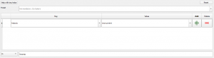
- Go to the Vector menu, and open the “QuickOSM” tool you have just installed. This will open a window that allows you to search for features of interest to you.
- In the “Key” dropdown menu, you can choose the broad category of features you are interested in. Under “Value”, you can narrow this category down a little. You will also need to choose a location to download features for. In the example below, I am looking for monuments in Toronto.
- Scroll down the QuickOSM window to find the “Run query” button, and click this to execute your download.
- The data will automatically be added to your map, so you can close the QuickOSM window if you are finished with it.
- If you don’t see any data on your map, try right clicking on the dataset in the layers panel, and clicking “Zoom to layer”.
- If you wish to save your dataset permanently to your computer, right click on its name in the layers panel, and choose “Make permanent”. Save your data as an ESRI shapefile in a location where you will be able to find it again later.
Making Spatial Data Files More Manageable
Often, spatial data files are very large. In the GeoHub section, for example, you downloaded the roads for all of Ontario. You may have found this file was slow to load, and that it took up a lot of space on your computer. You may also have found that the roads covered an area larger than you really wanted to map, or that you were only interested in highways, and not all of the other roads. Any of these are good reasons to try and decrease the size of your spatial data file. One way of reducing the file size is simply to remove features that you don’t actually need.
There are two basic methods to do this. Exporting takes a subset of your original file based on the attributes of each feature (only roads labelled highway, for example), and puts that subset into a new file. Attributes are a key component of spatial data; if you need a review on what they are, refer to Appendix 1. Once you have your subset file, you could delete the original to free up space, or remove it from the GIS project to prevent lagging.
The other basic method is clipping. When you clip, you need two files; the one you want to remove features from, and another which determines the features that will be kept. So, for example, if you wished to remove all roads that weren’t in the city of Ottawa, you would need the road file, and a file representing the boundary of Ottawa. When you run the clip, any roads inside the Ottawa boundary would be placed into a new file.
Exporting
For this example, we will use the provincial park boundaries downloaded from GeoHub in6 the API section of this lab. This technique can be applied to any spatial data that has multiple features. In fact, it is equivalent to the filtering step described in the GeoHub instructions, and is a useful alternative if your filtered file is taking too long to create.
- Make sure the shapefile you want to subset is open in QGIS. Click on its name in the layers panel to highlight it.
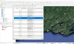
- Press F6 on your keyboard to open the attribute table.
- For now, we will simply select features manually. In the table, click the grey bar to the side of the feature you would like to export. I have chosen Presqu’ile Provincial Park. Note that there are several other ways of selecting features, including by writing an expression, by their spatial relationship to another shapefile, or by clicking them on the map. QGIS provides helpful documentation if you would like to give these methods a try [https://docs.qgis.org/3.16/en/docs/user_manual/introduction/general_tools.html#selecting-features].
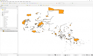
- Once you have selected the features you want to export, return to the main QGIS window. In the layers panel, right click on the name of your file, and from the Export menu choose “Save Selected Features As”.
- Choose a file type (as with the rest of the lab, we recommend that you use ESRI Shapefile), and an appropriate name and location for the new file. Then click “OK” to export the file.
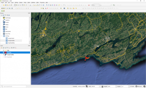
The new file should be loaded into your map automatically, but if not, simply drag and drop it from the browser panel.
Clipping
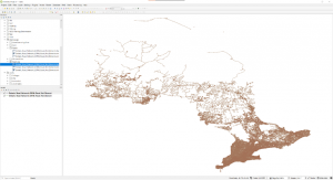
In this section, we will clip a layer of Ontario trail segments downloaded from GeoHub; you may choose whether to download the files manually or use an API, but you should note that API downloads can be a little glitchy for files containing large numbers of features. We will use Presqu’ile provincial park as our boundary, and create a file containing only those trails inside the park.
- Load both of your datasets into QGIS if you haven’t already.
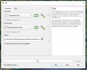
- In the Vector menu at the top of the screen, open the Geoprocessing Tools sub-menu and click “Clip”.
- Set your “Input layer” to be your trails (the features you wish to trim) and your “Overlay layer” to be the park (the features you want to do the trimming with).
- Use the “…” button next to the “Clipped” text box to choose your output type. If you might need your clipped file again, it’s best to save to file. Choose an appropriate output name and location, and set the file type to “SHP files”.
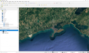
- Click run. The file will automatically be added to your map once it is complete, but the clip window will not close automatically.
Assignment
Using QGIS, make a basic map with data from Open Street Map and at least one of the other sources described in this lab. Take a screenshot of your map, and submit it along with a brief description of some critical considerations relating to your non-OSM data source. This should include information on who produced the dataset, what methodologies were used, and what the original purpose of the data may have been. You should also include a few ideas about how this data could be used in a counter mapping context.
References
Textual References
Jefferson, Brian Jordan. “Predictable Policing: Predictive Crime Mapping and Geographies of Policing and Race,” Annals of the American Association of Geographers 108, no. 1 (2018): 1-16. DOI: 10.1080/24694452.2017.1293500
Peluso, Nancy Lee. “Whose Woods are These? Counter-Mapping Forest Territories in Kalimantan, Indonesia,” Antipode 27, no. 4 (1995): 383-406. DOI: 10.1111/j.1467-8330.1995.tb00286.x
Images
“Home,” Ontario GeoHub. Accessed January 13, 2022.
“Ontario Road Network (ORN) Road Net Element Item Page,” Ontario GeoHub. Accessed January 2013, 2022.
“Search Results,” USGS EarthExplorer. Accessed January 13, 2022.
Data Used in this Lab
“Boundary Files,” 2016 Census. Shapefile. Ottawa, ON: Statistics Canada (2016). Catalogue no. 92-160-X.
Historic Monuments. Shapefile. OpenStreetMap Users, January 13, 2022.
Ontario Road Network (ORN) Road Net Element. Shapefile. Peterborough, ON: Ontario Ministry of Natural Resources and Forestry, September 27, 2019.
Ontario Trail Network (OTN) Segment. Shapefile. Peterborough, ON: Ontario Ministry of Natural Resources and Forestry, January 13, 2021.
Basic GIS Concepts Covered in this Lab
Since this lab teaches you to download spatial data, it may be helpful to define this term. You can probably find a wide range of definitions online, but for the purposes of this course, spatial data are data that refer to a specific location; that is, we know their location in space. They can describe a wide range of properties of that location, including its history, physical features, and demographics. The things about a location which are being described are generally called attributes, and are stored in a table attached to your spatial data. Each row of the table will contain the attributes of a different location.
There are a wide variety of spatial data formats. In this lab, you are asked to work mainly with shapefiles. These have the extension .shp, and were originally developed by ESRI. They have now become one of the most widely used spatial data formats in circulation, though they have their downsides. They can’t be used to store data made up of pixels, such as satellite imagery or other photographs, for example. They also can’t exceed a certain file size. For this lab, however, the most important downside is that they are actually made up of multiple files, all of which must be stored together in order to work. If you accidentally delete one of these files, or if you forget to move all of them together, your spatial data may no longer open.
Some Optional Readings
The Power of Maps
Crampton, Jeremy. “Maps as social constructions: power, communication and visualization,” Progress in Human Geography 25, no. 2 (2001): 235-252. DOI: 10.1191/030913201678580494. https://journals.sagepub.com/doi/pdf/10.1191/030913201678580494
Hunt, Dallas & Shaun Stevenson “Decolonizing Geographies of Power: Indigenous Digital Counter-mapping Practices on Turtle Island,” Settler Colonial Studies 7, no. 3 (2016). 1-21. DOI: 10.1080/2201473X.2016.1186311. https://www.researchgate.net/publication/304069759_Decolonizing_geographies_of_power_indigenous_digital_counter-mapping_practices_on_turtle_Island/citation/download
Counter Mapping
Dalton, Craig M. & Tim Stallmann. “Counter-Mapping Data Science,” The Canadian Geographer 62, no. 1 (2018): 93-101. DOI: 10.1111/cag.12398. https://www.countercartographies.org/wp-content/files/Dalton_counter-mapping_data_science.pdf
Hodgson, Dorothy L. & Richard A. Schroeder. “Dilemmas of Counter-Mapping Community Resources in Tanzania,” Development and Change 33, no. 1 (2002): 79-100. DOI: 10.1111/1467-7660.00241. https://www.semanticscholar.org/paper/Dilemmas-of-counter-mapping-community-resources-in-Hodgson-Schroeder/f9d8609e01ef2dee2311eb6d7ce30ac70d71cd0f
O’Dwyer, Laurence. “Counter-Mapping: Cartography that Lets the Powerless Speak,” Guardian (March 6, 2018). https://www.theguardian.com/science/blog/2018/mar/06/counter-mapping-cartography-that-lets-the-powerless-speak
