In the previous chapter we learned that Reich (1971) wanted to measure the degree of discrimination between two groups by comparing their wages.  He took the entire difference in wages to be the result of discrimination.  He basically said, “even if some of the non-minority wage premium is due to higher education, the fact that non-minorities have higher education is due to discrimination also.”

Schiller (1973) agreed with Reich that the wage gap is all due to discrimination, estimating that about one half the White:Black wage gap in 1970 was due to past discrimination in education and housing, one quarter was due to past discrimination by employers resulting in lower work skills and experience, and one quarter was due to current discrimination against Black people regardless of their education, housing, current work skills, or experience.

We can think of the wage gap is being made up of two factors, achievement differences (possibly due to past discrimination as per Reich and Schiller), and current discrimination that rewards achievement differently depending racial or other identity.

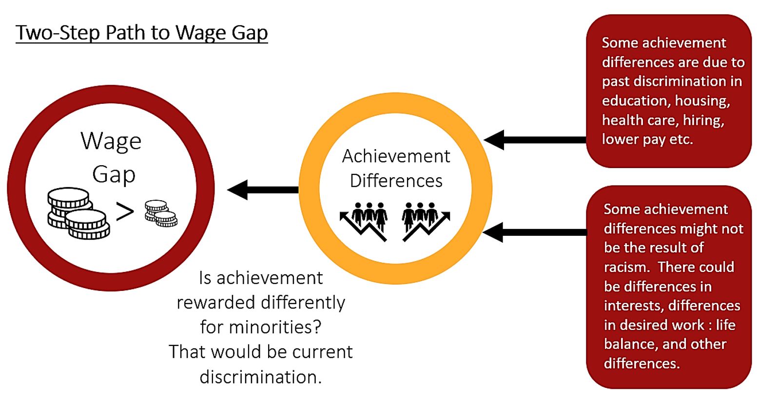
The figure above shows a two-step path to the wage gap.  First, each group achieves different levels of education, health, skills, experience, and other relevant characteristics.  Second, each group is offered a wage supposedly based on those achievements. Discrimination can occur at each step.  We will quantify these two effects using Econometrics.

What is Econometrics?

Econometrics is the use of statistics to model, explain and predict economic data. Its most powerful tool is regression analysis. Regression analysis finds best-fit lines or equations to describe data, as though the dependent variable  is a function of various explanatory variables.

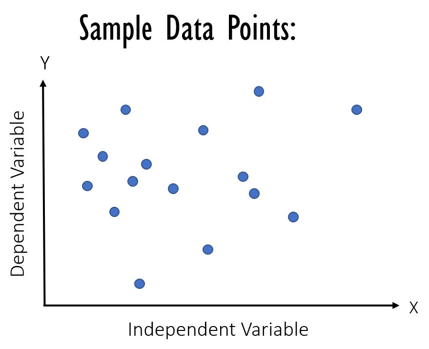
For example, if we had data on weight and height for many individuals, we could run a regression which tries to relate weight (the dependent variable) to height (the explanatory variable or independent variable).

The regression software would find a best-fit line through all the data points, something like: W_i = 90 + 1.05 H_i + ε_i (with weight in pounds and height in inches) where W_i is the weight of person i, 90 is the vertical intercept (representing 90 pounds), and H_i is the height of that same individual. 1.05 is the coefficient in front of H, meaning it is the slope of the best-fit line; it is the marginal effect of height on weight. We can’t really think of it as the degree to which height explains weight, because it will be a different size depending on which units we use for height, whether inches or centimeters or whatever. ε_i is a random error for person i representing something about person i’s weight that we can’t explain.

Not all observations, not all people will be on the best-fit line. When 90 + 1.05 H_i is not the same as W_i, we call the difference the error, ε_i. Using the equation of the best-fit line, we “explain” weight in terms of height. And we can also predict your weight based on your height. The expectation of your weight using your height is just 90 + 1.05 * your height.

Have we proved that height causes weight?

In the example above, we used just one independent variable to explain weight. In real life, your weight depends on more than just your height.  It depends on your age, your gender, and the calories you consume each day. Regression analysis can handle that. Regression analysis can compute a multi-dimensional best-fit line, a best-fit space.

Best-fit:

How does the regression analysis software find the best-fit line or best-fit space? The most basic technique is called ordinary least squares (OLS). In OLS, the software finds the line which minimizes the distance between itself and the data points.

More precisely, the best-fit line is the line that minimizes the sum of squared deviations from the line; that is, the line that minimizes the sum of squared errors.

A “deviation” is the error ε_i , the difference between our dependent variable, call it Y, and our expectation of what Y will be based on the explanatory variables.

The “hat” sign above the Y stands for expectation, or estimate. Why do we square the deviations?

Two reasons. First, we don’t care if the deviation is positive or negative, below the line or above it. They both matter and we don’t want to subtract the negative ones from the positive ones. Squaring means we are counting them all.

Second, we care more about the really far out mistakes than the slight mistakes.  Squaring makes the really far out deviations count more.

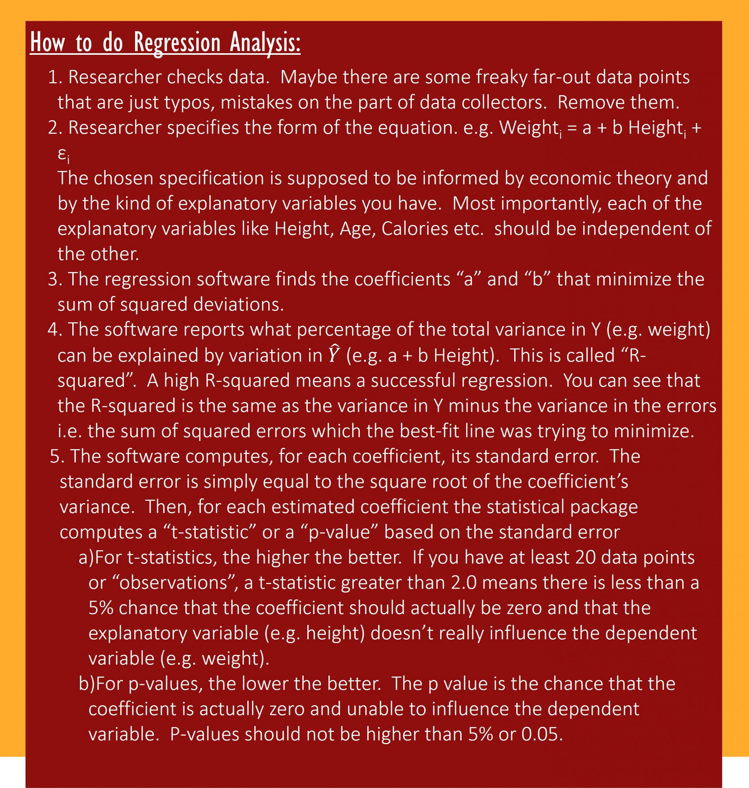
Here is a checklist for performing regressions.

Dummy Variables:

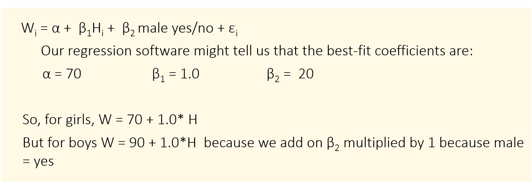
Sometimes we want to use qualitative information in our regression. In our Weight regression example, we could use Gender to explain weight, not just Height. But what number do we type in for Gender?

Qualitative variables like Gender become “dummy variables”, either equal to one or to zero. In the case of Gender, we ask if the person is male yes/no. Or we could ask if the person is female yes/no. Either way. If the answer is yes, we type in “1”. And if the answer is no, we type in “0”.

Let’s say we perform the regression:

An Example from Automobile Insurance:

Robinson, Sloan, and Eldred (2018) use a regression to relate the probability of a car accident to driver characteristics which are known by the insurance company. They used data from four American states in 2010-2012. Their results are displayed below.

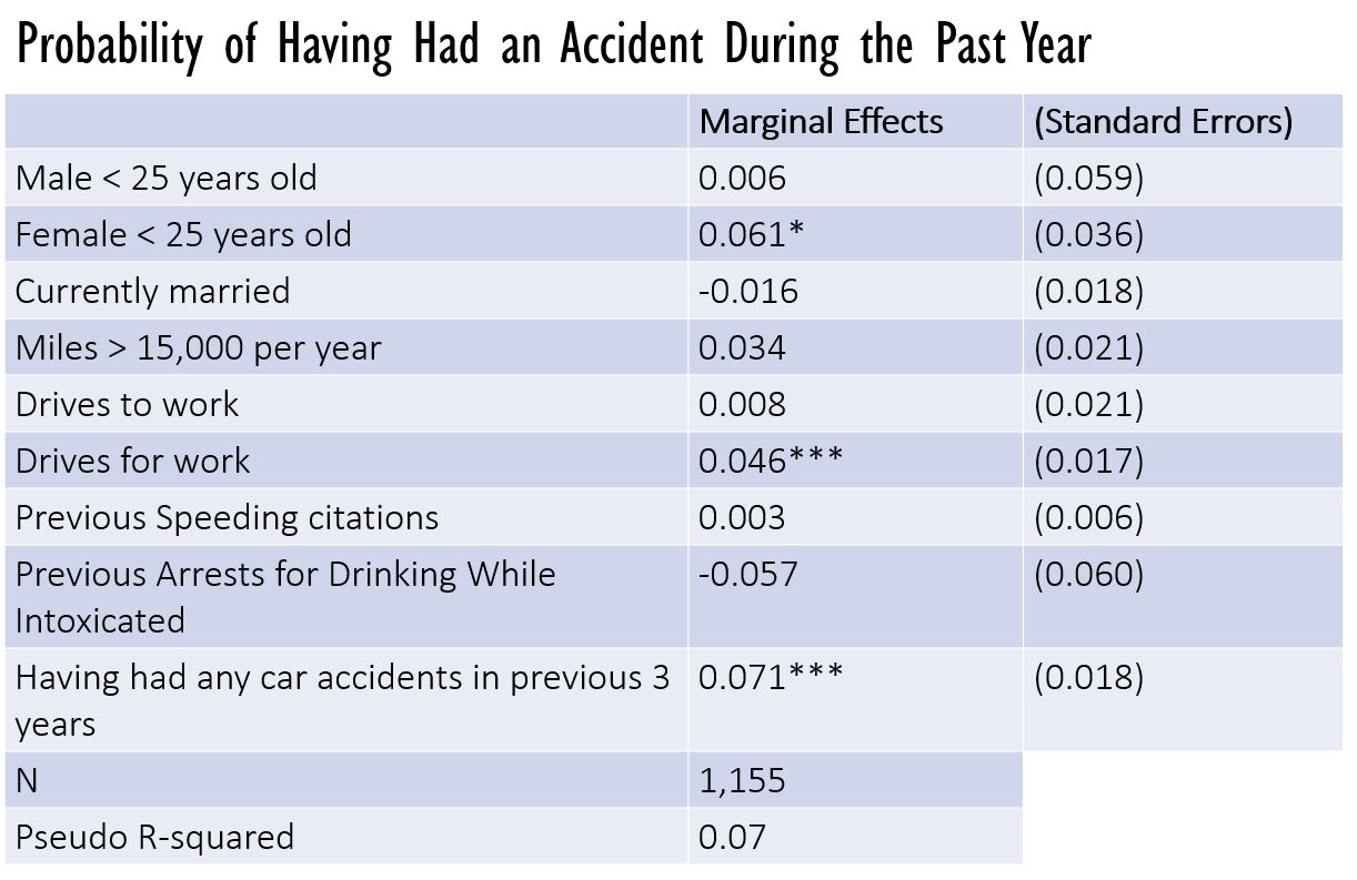
The N tells us that there were 1,155 data points, 1,155 people in the study. The R-squared is very low, suggesting that some important explanatory variables have been left out of the regression. It’s called a “Pseudo” R-squared as this is a different kind of regression, where the dependent variable is a dummy variable  (accident yes = 1, accident no = 0).

We see that being a young man is positively correlated with having an accident. But look at the standard error! It is just about the same size as the coefficient, the marginal effect.  So we can’t really be sure about the correlation.

When we look at young women, we see an effect that is larger in relation to its standard error.  It has an asterisk next to it, indicating that its p value is less than 0.10.  That means that there is less than a 10% chance that this is a false positive. That’s still higher than the 5%-or-less chance we like to see, though, so we don’t put much confidence in this correlation.

Driving for work, and having had a car accident in the previous three years, are correlations we can be more confident about. They are more statistically significant predictors of having had a car accident in the past year. They have three asterisks next to them, indicating a p value of less than 0.01.

Professor Feir’s Study of Earnings and Discrimination:

Donn Feir (2013), for a paper entitled, Size, Structure, and Change: Exploring the Sources of Aboriginal Earnings Gaps in 1995 and 2005, collected data on Canadians aged 25-55 who make more than $100 per year in wages and salaries. With that data, they compared the yearly earnings of Métis, and Status persons living off reserve to the yearly earnings of non-minority Canadians. Just using the fact that annual earnings is equal to weekly earnings multiplied by the number of weeks worked, Feir found that about half the gap between the two groups was due to Métis and Status persons working fewer weeks per years than non-minority Canadians.

Then, using 1995 and also 2005 data, Feir analyzed the weekly earnings of different racial groups when they were employed. They found, first of all, that the Indigenous weekly earnings were lower than the weekly earnings of non-Indigenous, non-immigrant, non-minority Canadians. Non-Indigenous, non-immigrant, and non-minority men made 36% more than First Nations-identifying men who live off reserve.

(On a happier note, data from TD Bank^[1] indicates that the wages of Indigenous people grew faster than those of non-Indigenous people between 2007 and 2014.  In 2014 Indigenous men had an average weekly wage of $973 compared to $1,024 for non-Indigenous; Indigenous women had $697 compared to $773.)

Feir’s Analysis

Feir then asked how much of the difference in weekly earnings between Indigenous and non-Indigenous workers was due to differences in characteristics like age, education, number of children, language spoken, and other explanatory variables. How much of the weekly earnings gap was due to differences in characteristics, and how much was due to those characteristics being rewarded differently depending on race?

Comparing First Nations men off-reserve to non-minority Canadians, Feir found that about half the difference in weekly earnings in 2005 was due to characteristics being rewarded differently. It was the same for women.

Comparing First Nations off-reserve to First Nations on-reserve, 90% of the difference for men was due to difference in rewards, and 84% of the difference for women was due to difference in rewards.

How did Feir calculate this? A technique called Blinder Oaxaca Decomposition was used.

Blinder-Oaxaca Decomposition (BOD):

BOD involves running two regressions, one for the minority group, and one for the non-minority. With the data for the two groups, and the coefficients estimated by the software for the two groups, you can separate the wage gap into its two components – differences in achievement, and differences in how achievement is rewarded.

Here is a simple example using data collected by a group of students at Queen’s University for various First Nations and municipalities of similar size and location in Ontario. The data excludes fly-in communities.

Here are the average values of the data used in the regressions:

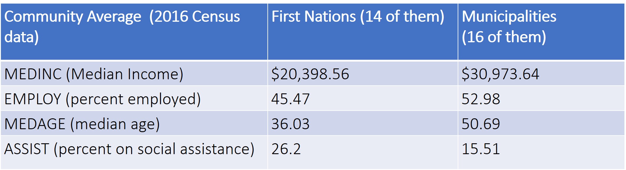
As you can see from the Table above, First Nations in the sample had lower median income, lower employment rates, lower median age, and higher rates of social assistance compared to municipalities.

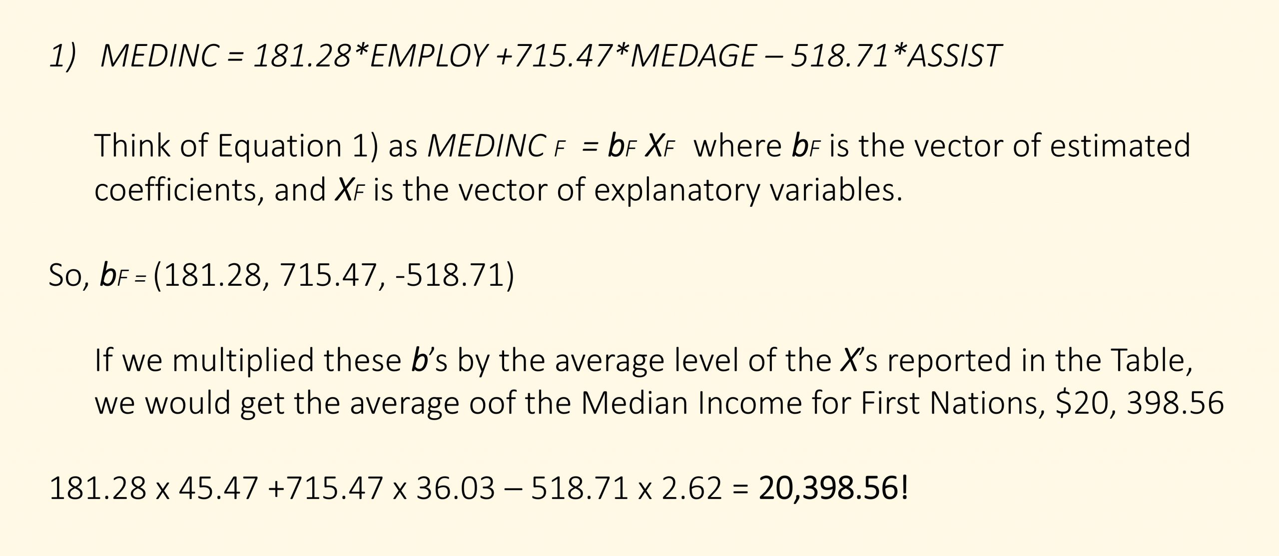
Now let’s run two regressions, one for the First Nations and one for the municipalities. In each regression, median income is the dependent variable which we are trying to explain, and the explanatory variables are percentage of the community’s adults^[2] employed, median age, and percentage of the community’s adults on social assistance. Those explanatory variables are the “characteristics” or “achievements”. Each regression, one for the First Nations, and one for the municipalities, generates coefficients which show the marginal effect of each characteristic on the group’s median income.

It is questionable whether EMPLOY and ASSIST are truly independent of one another, as independent variables should be; however, let us proceed as though they were tested and found to be sufficiently independent.

The First Nations regression yields the following output:

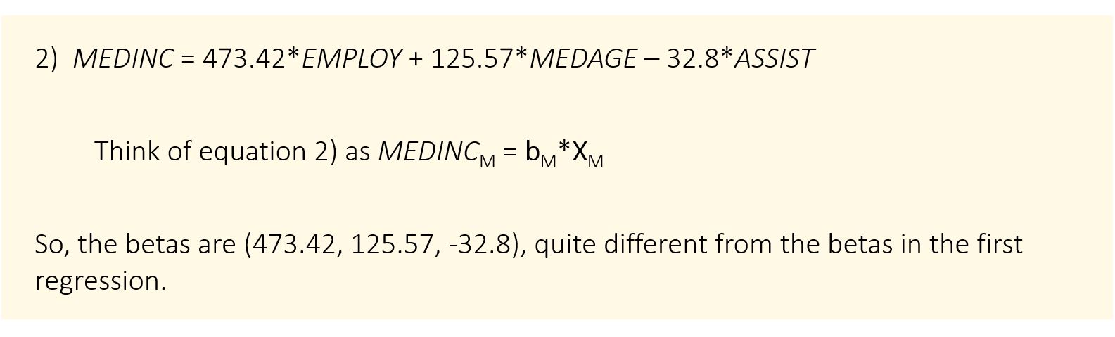
For Municipalities, a regression yields:

Blinder and Oaxaca showed that, assuming that First Nations, but not Municipalities, are experiencing discrimination, we ignore interaction effects and write the difference in average MEDINC this way:

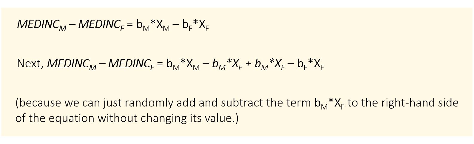
Rearranging,

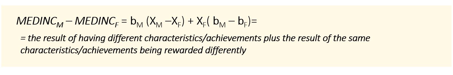
This equation tells us that the difference in median income between the two kinds of communities depends not only on the differences in the Xs (i.e. differences in employment rates, age, social assistance levels) but also on the fact that, even if the communities had exactly the same Xs, the betas of the municipalities differ from the betas of the First Nations and translate characteristics into a higher level of median income.

Is that because of discrimination? We can’t be sure. We have left some relevant explanatory variables out of our regression, and our omissions could result in this apparent failure to reward characteristics equally for First Nations and municipalities.

Looking at the difference in the coefficients for the two groups, we see that municipalities seem to benefit more from employment and be hurt less by social assistance rates, for no obvious reason.

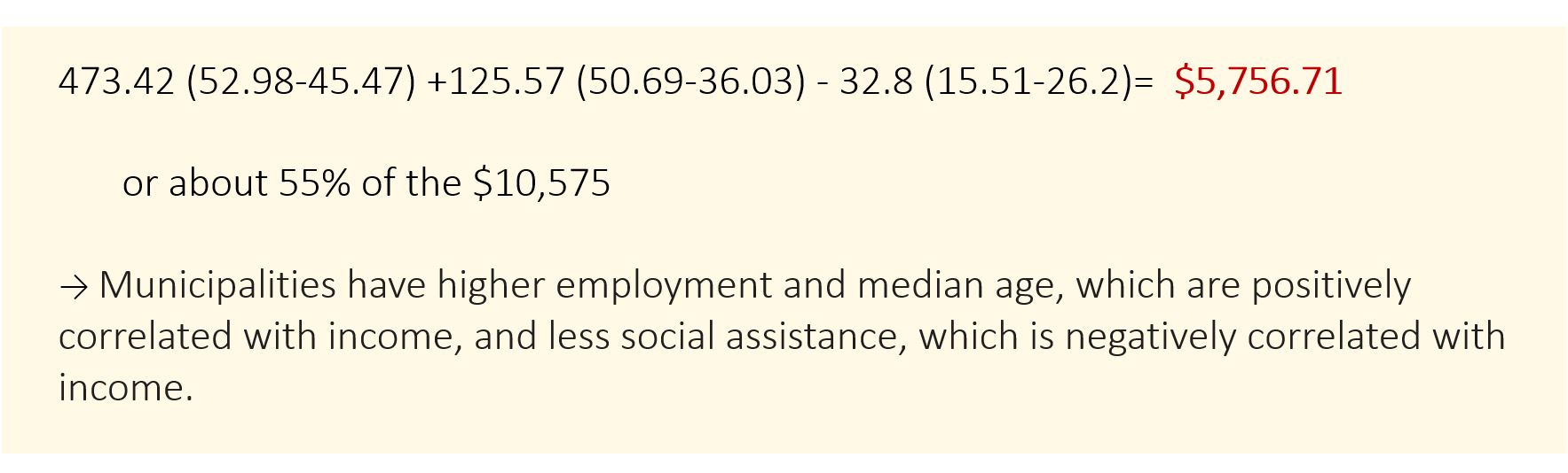
Let’s compute some actual numbers. Difference between MEDINC for the two kinds of communities:

So the average First Nation in this sample has a median income more than $10,000 below the average Municipality in this sample.

We’re about to calculate the fact that only 55% of that difference can be explained by differences in levels of employment, median age, and social assistance.

First, we calculate the difference in achievements between Municipalities and First Nations using b_M (X_M –X_F):

Second, we calculate the difference in the way achievements are rewarded using X_F (b_M – b_F):

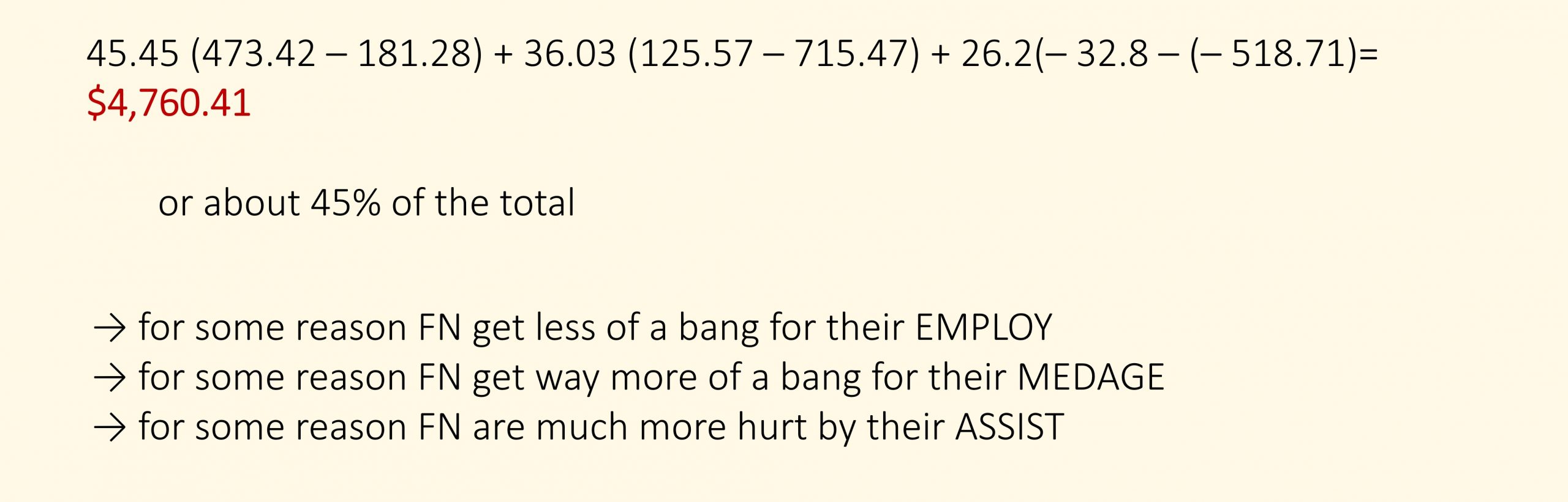
So, there is a significant gap in median income between these Ontario municipalities and reserves.  55% of that gap comes from differences in characteristics (employment, median age, and social assistance rate). 45% of the income gap comes from different rewards for employment, median age, and social assistance.

We have now seen how regression analysis and Blinder-Oaxaca Decomposition can be employed to make sense of wage gaps, pointing to likely channels of discrimination. We now leave our study of discrimination and return to our chronology of the Indigenous experience in Canada.