8.6 Exponential Functions
Consider these two companies:
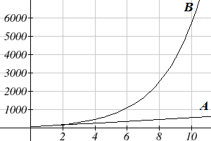
- Company A has 100 stores, and expands by opening 50 new stores a year
- Company B has 100 stores, and expands by increasing the number of stores by 50% of their total each year.
Company A is exhibiting linear growth. In linear growth, we have a constant rate of change – a constant number that the output increased for each increase in input. For company A, the number of new stores per year is the same each year.
Company B is different – we have a percent rate of change rather than a constant number of stores/year as our rate of change. To see the significance of this difference compare a 50% increase when there are 100 stores to a 50% increase when there are 1000 stores:
- 100 stores, a 50% increase is 50 stores in that year.
- 1000 stores, a 50% increase is 500 stores in that year.
Calculating the number of stores after several years, we can clearly see the difference in results.
| Years | Company A | Company B |
| 2 | 200 | 225 |
| 4 | 300 | 506 |
| 6 | 400 | 1139 |
| 8 | 500 | 2563 |
| 10 | 600 | 5767 |
This percent growth can be modeled with an exponential function.
Exponential Function
An exponential growth or decay function is a function that grows or shrinks at a constant percent growth rate. The equation can be written in the form [latex]f(x)=f_0(1+r)^x[/latex] or [latex]f(x)=f_0\cdot b^x[/latex] where [latex]b=1+r[/latex].
Here:
- [latex]f_0[/latex] is the initial or starting value of the function,
- [latex]r[/latex] is the percent growth or decay rate, written as a decimal (note that [latex]r[/latex] is a negative number in the case of rate of decay),
- [latex]b[/latex] is the growth factor or growth multiplier. Since powers of negative numbers behave strangely, we limit [latex]b[/latex] to positive values.
Example 1 – Exponential Growth
India’s population was 1.14 billion in the year 2008 and is growing by about 1.34% each year. Write an exponential function for India’s population, and use it to predict the population in 2020.
Answer: Using 2008 as our starting time ([latex]t = 0[/latex]), our initial population will be 1.14 billion. Since the percent growth rate was 1.34%, our value for [latex]r[/latex] is 0.0134. Let [latex]P[/latex] represent India’s population size (in billions).
Using the basic formula for exponential growth [latex]P(t)=a(1+r)^t[/latex] we can write the formula, [latex]P(t)=1.14(1+0.0134)^{t}[/latex]
To estimate the population in 2020, we evaluate the function at [latex]t = 12[/latex], since 2020 is 12 years after 2008: [latex]P(t)=1.14(1+0.0134)^{12}\approx 1.337 \text{ billion people in India in 2020.}[/latex]
Example 2 – Exponential Decay
A cell phone company is introducing to the market a new model for a cell phone and needs to plan how long the should keep manufacturing and selling the current model before taking it off the market. Market analysis and the analysis of their sales trends with previous “old” models suggests that the sales of the current model will decrease by 12.34% annually while their current sales are at 259.37 million. Create the function model that represents the number [latex]n[/latex] of current model cell phones sold (in millions) each year [latex]t[/latex] years from now and estimate the annual sales of the current models 5 years from now.
Answer: [latex]n(t)=?, n(5)=?[/latex], [latex]n[/latex] decreasing by % per year [latex]\rightarrow[/latex] exponential decay
[latex]\rightarrow[/latex] number of phones sold each year is 100%-12.34%=87.66% of the number of phones sold the previous year, with 259.37 million at the start, so we have:
[latex]\begin{align*} n(0)&=259.37\\ n(1)&=259.37(1-0.1234)=259.37(0.8766)\\ n(2)&=n(1)(1-0.1234)=n(1)(0.8766)=259.37(0.8766)(0.8766)\\ &=259.37(0.8766)^2\\ n(3)&=n(2)(1-0.1234)=n(2)(0.8766)=259.37(0.8766)^2(0.8766)\\ &=259.37(0.8766)^3 \end{align*}[/latex]
etc. Therefore,
[latex]n(t)=259.37(0.8766)^t,\ \ \ \ \ \ t>0[/latex]
In particular, five years from now, [latex]t=5[/latex] and so
[latex]n(5)=259.37(0.8766)^5\approx 134.25[/latex]
Therefore, five years from now, the annual sales of the current model would be approximately 134.25 million.
Important note: how to distinguish between linear and exponential change?
If a quantity is changing by a fixed amount over equal periods, the change is linear.
If a quantity is changing by a percentage rate over equal periods, the change is exponential.
Example 5 – interpreting components of an exponential function
Suppose that [latex]T(q)[/latex] represents the total number of Android smart phone contracts, in thousands, held by a certain Verizon store region measured quarterly since January 1, 2015. Interpret all of the parts of the equation [latex]T(2)=86(1.64)^2=231.3056[/latex] .
Answer: Considering [latex]T(2)[/latex], we know that it represents the total number of Android smart phone contracts, in thousands, held by the given Verizon store region after [latex]2[/latex] quarters, i.e., after 6 months.
Interpreting the rule for calculating [latex]T(q)[/latex], we can see that it is an exponential function, with 86 as our initial value. This means that on Jan. 1, 2015 this region had 86,000 Android smart phone contracts.
Since the growth factor is [latex]b = 1 + r = 1.64[/latex], we know that every quarter the number of smart phone contracts grows by 64%.
Therefore, [latex]T(2) = 231.3056[/latex] means that in the second quarter (or at the end of the second quarter) there were approximately 231,306 Android smart phone contracts.
Periodic Compound Interest
In finance, a common way to apply interest, whether borrowing or lending, is by compounding. The term “compounding” means that some quantity is being added on top of another before calculating the overall effect.
Linguistically, we may say “my problems are compounding”. That means that the problems are not just simply adding up, but that problem number 2 is making problem number 1 more complicated, so the overall result is a more complex problem than just the two problems combined.
Mathematically, when we talk about a periodic compounding interest rate, it means that the interest earned during a specific period is added to the current amount and then the interest for the next period is calculated based on this larger amount because it now also includes the interest earned during the previous period.
When we talk about interest rates, they are typically expressed as annual rates, or % per year. However, if the interest is compounded over a number periods every year, then this rate is equally divided by the number of periods per year to give us the periodic interest rate, before being applied to the current amount in the investment (or a loan) for that period. Mathematically, we can calculate the total amount of an investment (or a loan) compounded at a particular annual frequency and at a particular annual rate after a specific number of years as follows:
Periodic compounding interest formula
[latex]\text{total amount (incl. interest)}=(\text{starting amount})\left(1+\frac{\text{annual rate}}{\text{# comp. periods per year}}\right)^{(\text{# comp. periods per year})(\text{# years})}[/latex]
or
[latex]A=P\left(1+\frac{r}{m}\right)^{mt}[/latex]
where
[latex]A[/latex] is the total amount of the investment or the loan
[latex]A_0[/latex] is the initial, or present, amount of the investment or the loan
[latex]r[/latex] is the annual rate of interest
[latex]m[/latex] is the compounding frequency, i.e., number of compounding periods per year
[latex]t[/latex] is the number of years
important note: the value for time [latex]t[/latex] in periodic compounding must be rounded down, if necessary, to the end of the last period in the overall time frame. This is because no additional interest is earned during the last period until the period ends. For example, if compounding quarterly, the overall time of 2 years and 4 months must be rounded down to 2 years and 3 months because that would be the end of the last quarter in the overall time. During the 4th month no additional interest is earned because the next quarter is not yet complete.
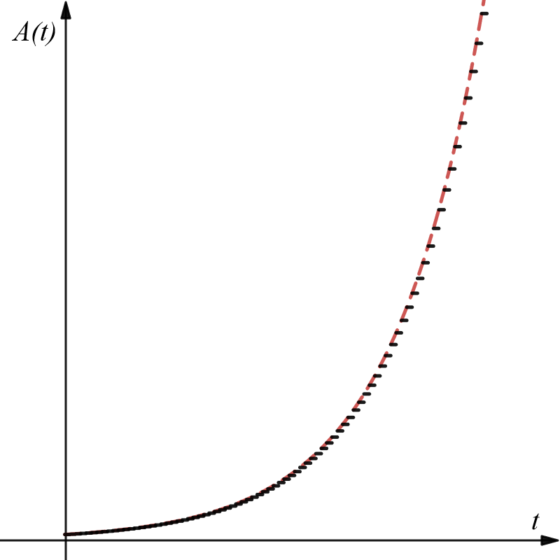
Note that [latex]A[/latex] will change as time [latex]t[/latex] changes, and so we can think of [latex]A[/latex] as a function of [latex]t[/latex], i.e., [latex]A(t)[/latex]. Note also that [latex]A(t)[/latex] is not quite an exponential function, but it behaves like one on the end points of the compounding intervals. See the general graph of [latex]A(t)[/latex] below as an illustration of this:
Example 4 – periodic compounding interest
A certificate of deposit (CD) is a type of savings account offered by banks, typically offering a higher interest rate in return for a fixed length of time you will leave your money invested. If a bank offers a 24 month CD with an annual interest rate of 1.2% compounded monthly, how much will a $1000 investment grow to over those 24 months?
Answer: investment amount after 24 months?
[latex]\rightarrow A(t)=?, t=24 \text{ months}=2\text{years}\rightarrow A(2)=?[/latex]
monthly compounding [latex]\rightarrow[/latex] # comp. periods per year = 12
Therefore,
[latex]A(t)=P\left(1+\frac{r}{m}\right)^{mt}=1000\left(1+\frac{0.012}{12}\right)^{12t}[/latex]
And so
[latex]A(2)=1000\left(1+\frac{0.012}{12}\right)^{12\cdot 2}=1024.28[/latex]
Therefore, after 24 months, the account will have grown to $1024.28.
Continuously Compounded Interest
When working with exponentials, there is a special constant we must talk about. It arises when we talk about things growing continuously, such as continuous compounding, or natural phenomena like radioactive decay that happen continuously. It is the constant [latex]e[/latex], or Euler’s Number and has a special place in describing many phenomena in mathematics. Just like pi, or [latex]\pi[/latex], it has infinitely many non-repeating decimals and it is an irrational number, meaning it cannot be represented as a fraction. Your calculator will use different number of decimals to round [latex]e[/latex] to an approximate value, depending on your calculator settings, however typically we would approximate it as follows:
Euler’s Number: [latex]e[/latex]
[latex]e\approx 2.718282[/latex]
For those who are interested, note that the value of [latex]e[/latex] is calculated by increasing the exponent [latex]n[/latex] towards infinity in the following expression:
[latex]e=\left(1+\frac{1}{n}\right)^n\text{ as }n\to\infty[/latex]
You can try it out yourself by calculating the above expression for increasingly larger values of [latex]n[/latex]. Note also that this is the same calculation as the growth portion of a periodic compounded interest where the annual rate is 100% and the frequency of compounding approaches infinite times per year.
Because [latex]e[/latex] is often used as the base of an exponential, most scientific and graphing calculators have a key that can calculate powers of [latex]e[/latex], usually labeled [latex]e^x[/latex]. Some computer software instead defines a function exp(x), where exp(x) = [latex]e^x[/latex]. Since calculus studies continuous change, we will almost always use the [latex]e[/latex]-based form of exponential equations in this course.
Continuous Growth Formula
Continuous growth can be calculated using the formula [latex]f(x)=ae^{rx}[/latex] where
- [latex]a[/latex] is the starting amount,
- [latex]r[/latex] is the continuous growth rate.
A special case of this is the continuous compounding interest amount formula that calculates the amount [latex]A[/latex], including interest, after [latex]t[/latex] years:
[latex]A(t)=Pe^{rt}[/latex]
where [latex]P[/latex] is the initial amount (present value) and [latex]r[/latex] is the annual interest rate.
Example 5 – continuous compounded interest
Although typically, in everyday financial life, interest is compounded periodically, in economics we often use continuous compounding to ensure consistency between different calculations.
In this example, calculate the amount of interest on an investment of $2,000 after 10 and 5 months at the annual rate of 1.89% if compounded quarterly and if compounded continuously. Compare the two amounts of earned interest and explain briefly where the difference comes from within the context of how the interest is calculated.
Answer: interest = ?, interest = total amount – initial amount
compounded quarterly, so must round time down to nearest quarter period:
time = 10 years and 5 months [latex]\rightarrow[/latex] 10 years + 1 quarter [latex]t=10+\frac{3}{12}=10.25[/latex] years
[latex]\begin{align*} A_q(t)&=A_0\left(1+\frac{r}{m}\right)^{mt}\\ &\Rightarrow A_q(10\text{ years}, 5\text{ months})=2000\left(1+\frac{0.0189}{4}\right)^{4\cdot 10.25}=2426.42 \end{align*}[/latex]
Therefore, the amount of interest earned through quarterly compounding is $2,426.42 – $2,000 = $426.42.
compounded continuously, so must use exact time:
time = 10 years and 5 months [latex]\rightarrow t=10+\frac{5}{12}[/latex] years
[latex]\begin{align*} A_c(t)&=P\cdot e^{rt}\\ &\Rightarrow A_c(10\text{ years}, 5\text{ months})=2000\cdot e^{0.0189\cdot \left(10+\frac{5}{12}\right)}=2435.18 \end{align*}[/latex]
Therefore, the amount of interest earned through continuous compounding is $2,435.18 – $2,000 = $435.18.
More interest is earned through continuous compounding because the interest earned is being reinvested on top of the principal (or the initial) amount more frequently (infinitely more frequently, in fact) when compounding continuously than when compounding quarterly.
Graphs of Exponential Functions
Graphical Features of Exponential Functions
Graphically, in the function [latex]f(x)=a\cdot b^x[/latex].
- [latex]a[/latex] is the vertical intercept of the graph.
- [latex]b[/latex] determines the rate at which the graph grows:
- the function will increase if [latex]b \gt 1[/latex],
- the function will decrease if [latex]0 \lt b \lt 1[/latex].
- The graph will have a horizontal asymptote at [latex]y = 0[/latex].
- The graph will be concave up if [latex]a \gt 0[/latex]; concave down if [latex]a \lt 0[/latex].
- The domain of the function is all real numbers.
- The range of the function is [latex](0,\infty)[/latex] if [latex]a \gt 0[/latex], and [latex](-\infty, 0)[/latex] if [latex]a \lt 0[/latex].
When sketching the graph of an exponential function, it can be helpful to remember that the graph will pass through the points [latex](0, a)[/latex] and [latex](1, ab)[/latex].
The value [latex]b[/latex] will determine the function’s long run behavior:
- If [latex]b \gt 1[/latex], as [latex]x\to\infty[/latex], [latex]f(x)\to\infty[/latex], and as [latex]x\to -\infty[/latex], [latex]f(x)\to 0[/latex].
- If [latex]0 \lt b \lt 1[/latex], as [latex]x\to\infty[/latex], [latex]f(x)\to 0[/latex], and as [latex]x\to -\infty[/latex], [latex]f(x)\to \infty[/latex].
Example 6 – sketching graphs of exponential functions
Sketch a graph of [latex]f(x)=4\left(\frac{1}{3}\right)^x[/latex]
Answer:
This graph will have a vertical intercept at (0,4), and pass through the point [latex]\left(1,\frac{4}{3} \right)[/latex]. Since [latex]b \lt 1[/latex], the graph will be decreasing towards zero. Since [latex]a \gt 0[/latex], the graph will be concave up.
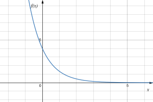
We can also see from the graph the long run behavior: as [latex]x\to\infty[/latex], [latex]f(x)\to 0[/latex], and as [latex]x\to -\infty[/latex], [latex]f(x)\to \infty[/latex].
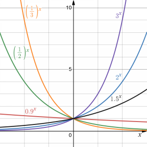
To get a better feeling for the effect of [latex]a[/latex] and [latex]b[/latex] on the graph, examine the sets of graphs below. The first set shows various graphs, where [latex]a[/latex] remains the same and we only change the value for [latex]b[/latex]. Notice that the closer the value of [latex]b[/latex] is to 1, the less steep the graph will be.
In the next set of graphs, [latex]a[/latex] is altered and our value for [latex]b[/latex] remains the same.
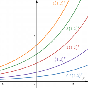
Notice that changing the value for a changes the vertical intercept. Since [latex]a[/latex] is multiplying the [latex]b^x[/latex] term, [latex]a[/latex] acts as a vertical stretch factor, not as a shift. Notice also that the long run behavior for all of these functions is the same because the growth factor did not change and none of these [latex]a[/latex] values introduced a vertical flip.
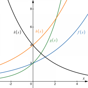
Example 7 – determining the graphs of exponential functions based on initial value and growth factor
Match each equation with its graph.
- [latex]f(x)=2(1.3)^x[/latex]
- [latex]g(x)=2(1.8)^x[/latex]
- [latex]h(x)=4(1.3)^x[/latex]
- [latex]k(x)=4(0.7)^x[/latex]
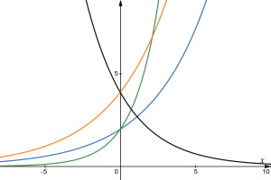
Answer:
The graph of [latex]k(x)[/latex] is the easiest to identify, since it is the only equation with a growth factor less than one, which will produce a decreasing graph. The graph of [latex]h(x)[/latex] can be identified as the only growing exponential function with a vertical intercept at (0,4). The graphs of [latex]f(x)[/latex] and [latex]g(x)[/latex] both have a vertical intercept at (0,2), but since [latex]g(x)[/latex] has a larger growth factor, we can identify it as the graph increasing faster.