8.2 Linear Functions
Section Exercises – after the reading
Work on section 8.2 exercises in Fundamentals of Business Math Exercises after reading this section. Discuss your solutions with your peers and/or course instructor.
You may consult answers to select exercises: Fundamentals of Business Math Exercises – Select Answers
As you hop into a taxicab in Allentown, the meter will immediately read $3.30; this is the “drop” charge made when the taximeter is activated. After that initial fee, the taximeter will add $2.40 for each kilometer the taxi drives. In this scenario, the total taxi fare depends upon the number of kilometers ridden in the taxi, and we can ask whether it is possible to model this type of scenario with a function. Using descriptive variables, we choose [latex]d[/latex] for distance in kilometers and [latex]C[/latex] for cost in dollars as a function of kilometers: [latex]C(d)[/latex].
We know for certain that [latex]C(0)=3.30[/latex], since the $3.30 drop charge is assessed regardless of how many kilometers are driven. Since $2.40 is added for each kilometer driven, we could write that if [latex]d[/latex] kilometers are driven, [latex]C(d)=3.30+2.40d[/latex] because we start with a $3.30 drop fee and then for each kilometer increase we add $2.40.
It is good to verify that the units make sense in this equation. The $3.30 drop charge is measured in dollars; the $2.40 charge is measured in dollars per kilometer. So
[latex]C(d)=3.30\text{ dollars}+\left(2.40\frac{\text{dollars}}{\text{kilometers}}\right) (d\text{ kilometers})[/latex]
When dollars per kilometer are multiplied by a number of kilometers, the result is a number of dollars, matching the units on the 3.30, and matching the desired units for the [latex]C[/latex] function.
Notice this equation [latex]C(d)=3.30+2.40d[/latex] consisted of two fixed quantities. The first is the fixed $3.30 charge which does not change based on the value of the input. The second is the $2.40 dollars per kilometer value, which is a rate of change in cost with respect to distance driven. In the equation this rate of change is multiplied by the input value.
Looking at this same problem in table format we can also see the cost changes by $2.40 for every 1 kilometer increase:
| [latex]d[/latex] | 0 | 1 | 2 | 4 |
| [latex]C(d)[/latex] | 3.30 | 5.70 | 8.10 | 10.50 |
It is important here to note that in this equation, the rate of change is constant; over any equal distance intervals, the change in cost is the same.
When graphing this function, the distance will be on the horizontal axis and the cost will be on the vertical because distance is the independent and cost is the dependent variable. When we graph the function we will see that the shape of [latex]C(d)=3.30+2.40d[/latex] is a line, which is how these types of functions get their name: linear functions.
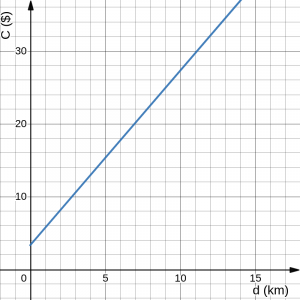
When the number of kilometers is zero, the cost is $3.30, giving the point (0, 3.30) on the graph. This is the vertical, or [latex]C[/latex]-, intercept. The graph is increasing in a straight line from left to right because for each kilometer the cost goes up by $2.40; this rate remains constant. Also note that, in this particular case, the line does not extend indefinitely on both sides. If we consider the domain of this function, i.e., the possible input values, we can see that although [latex]C(d)[/latex] can be (mathematically) calculated for any value of [latex]d[/latex], within the context of what [latex]d[/latex] and [latex]C(d)[/latex] represent, the value of [latex]d[/latex] cannot be negative.
Linear Function
A linear function is a function whose values change at a constant rate. The graph of a linear function produces a straight line.
Slope-Intercept Form of a Line
Linear functions can always be written in the form [latex]f(x)=mx+b[/latex] or [latex]f(x)=b+mx[/latex] where [latex]b[/latex] is the initial or starting value of the function (with input [latex]x = 0[/latex]), and [latex]m[/latex] is the constant rate of change of the function.
This form of a line equation is called slope-intercept form of a line.
Note that we conventionally use parameter names [latex]m[/latex] and [latex]b[/latex] in a general equation of a linear function, however they could be represented by any other name, as long as their meaning is defined in the context of the function. For example, the labour charge applied by a mechanic may be represented by [latex]C(t)=rt+I[/latex] where [latex]C[/latex] is the labour charge applied for work performed over [latex]t[/latex] hours at the rate of [latex]r[/latex] dollars per hour and with an initial charge of [latex]I[/latex] dollars.
Slope and Increasing vs. Decreasing
Given a line [latex]f(x)=mx+b[/latex], the number [latex]m[/latex] represents the constant rate of change of the function (called slope in the context of the graph of the function). The slope determines if the function is an increasing function or a decreasing function.
- [latex]f(x)=mx+b[/latex] is an increasing function if [latex]m\gt 0[/latex].
- [latex]f(x)=mx+b[/latex] is a decreasing function if [latex]m\lt 0[/latex].
If [latex]m=0[/latex], the rate of change is 0, and the function [latex]f(x)=0x+b=b[/latex] is just a horizontal line passing through the point (0, b), neither increasing nor decreasing.
Visual demonstration
Follow the link below to see the effect on the graph of a linear function [latex]f(x)=mx+b[/latex] while changing the value of rate of change parameter [latex]m[/latex] and the initial value [latex]b[/latex].
Example 1
Marcus currently owns 200 songs in his iTunes collection. Every month, he adds 15 new songs. Write a formula for the number of songs, [latex]N[/latex], in his iTunes collection as a function of the number of months, [latex]m[/latex]. How many songs will he own in a year?
Answer:
The initial value for this function is 200, since he currently owns 200 songs, so [latex]N(0)=200[/latex]. The number of songs increases by 15 songs per month, so the rate of change is 15 songs per month. With this information, we can write the formula
[latex]N(m)=15m+200[/latex]
Using the formula for [latex]N(m)[/latex], we can predict how many songs he will have in 1 year (12 months):
[latex]N(12)=200+15(12)=200+180=380[/latex]
Therefore, Marcus will have 380 songs in one year.
Concept Check
MathMatize: Reading and interpreting linear functions
Calculating Rate of Change
Because the rate of change in a linear function is constant, it is determined using the general relationship
[latex]m=\dfrac{\text{change in output}}{\text{change in input}}[/latex]
To calculate the change in output given the change in input, we need a pair of input and output values of the function. So if [latex]f(x)=mx+b[/latex] for some [latex]m[/latex] and [latex]b[/latex], then for any two distinct values for the input, [latex]x_1[/latex] and [latex]x_2[/latex], we get that
[latex]m=\dfrac{\text{change in output}}{\text{change in input}}=\dfrac{\Delta f}{\Delta x}=\dfrac{f(x_2)-f(x_1)}{x_2-x_1}[/latex]
Note that the symbol [latex]\Delta[/latex], read “delta”, is the upper case Greek letter for d, representing difference, or change.
Example 2
The population of a city increased from 23,400 to 27,800 between 2002 and 2006. Assuming that the population grew at a constant rate, find the rate of change of the population during this time span and interpret the result.
Answer:
In this relationship, the output is the size of the population and the input is the year. The rate of change will relate the change in output to the change in input, i.e., change in population to the change in time. The population increased by 27800-23400=4400 people over the 4 year time interval. To find the rate of change, or the change in the number of people per year:
[latex]\dfrac{\text{change in output}}{\text{change in input}}=\dfrac{27800-23400}{2006-2002}=\dfrac{4400}{4}=1100 \text{ people per year}[/latex]
This means that the population was increasing by 1100 people per year between 2002 and 2006.
(Note that we knew the population was increasing, so we would expect our value for the rate of change to be positive. This is a quick way to check to see if your value for the rate of change is reasonable.)
Example 3
Answer: In this relationship, the output is the pressure [latex]P[/latex] and the input is the depth [latex]d[/latex], and so [latex]P(d)[/latex] represents pressure at depth [latex]d[/latex].The rate of change, or slope, 0.434 represents the change in output in relation to the change in input, so the change in pressure in relation to the change in depth. Since the rate of change is positive, this tells us the pressure on the diver increases by 0.434 PSI for each foot their depth increases.
The initial value, 14.696, represents the value of [latex]P(0)[/latex], i.e., the pressure at 0 depth, so this tells us that at a depth of 0 feet, the pressure on the diver will be 14.696 PSI.
We can now find the rate of change given two input-output pairs, and could write an equation for a linear function if we had the rate of change and initial value. If we have two input-output pairs and they do not include the initial value of the function, then we will have to solve for it.
Example 4
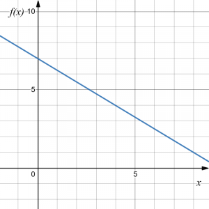
Determine the equation for the linear function graphed below.
Answer:
Looking at the graph, we can see that the input is [latex]x[/latex] and the output is [latex]f(x)[/latex] and that the line passes through the points (0, 7) and (4, 4). From the first point, we know that [latex]f(0)=7[/latex] and so the initial value of the function is [latex]b = 7[/latex]. In addition, the rate of change can be calculated as follows: [latex]m=\dfrac{\Delta\text{output}}{\Delta\text{input}}=\dfrac{4-7}{4-0}=\dfrac{-3}{4}=-\dfrac{3}{4}[/latex]
This allows us to write the equation for [latex]f(x)[/latex]: [latex]f(x)=-\frac{3}{4}x+7[/latex]
Example 5
If [latex]f(x)[/latex] is a linear function, [latex]f(3)=-2[/latex], and [latex]f(8)=1[/latex], find the equation for the function.
Answer:
The task is to determine the equation for [latex]f(x)[/latex].
The input is [latex]x[/latex] and the output is [latex]f(x)[/latex]. Since [latex]f(x)[/latex] is a linear function, it can be written as [latex]f(x)[/latex] for some values [latex]m[/latex] and [latex]b[/latex].
We are given two input-output pairs: (3,-2) and (8,1). Thus, the rate of change will be
[latex]m=\dfrac{\Delta\text{output}}{\Delta\text{input}}=\dfrac{f(8)-f(3)}{8-3}=\dfrac{1-(-2)}{8-3}=\frac{3}{5}[/latex]
Using the rate of change, we know the equation will have the form [latex]f(x)=\frac{3}{5}x+b[/latex].
In this case, we do not know the initial value [latex]f(0)[/latex], so we will have to solve for it. Since we know the value of the function when [latex]x = 3[/latex], we can evaluate the function at 3: [latex]f(3)=b+\frac{3}{5}(3)[/latex]. Since we know that [latex]f(3)=-2[/latex], we can substitute on the left side: [latex]-2=b+\frac{3}{5}(3)[/latex]. This leaves us with an equation we can solve for the initial value:
[latex]b=-2-\frac{9}{5}=-\frac{19}{5}[/latex]
Combining this with the value for the rate of change, we can now write a formula for this function:
[latex]f(x)=\frac{3}{5}x-\frac{19}{5}[/latex]
Example 5: Alternative solution (using math symbols)
Same problem as above. Compare step by step the text solution above with the solution below that uses primarily math symbols.
Answer:
Task: [latex]f(x)=?[/latex]
[latex]x[/latex] input, [latex]f[/latex] output, linear function
[latex]\Rightarrow f(x)=mx+b[/latex] for some [latex]m[/latex] and [latex]b[/latex].
[latex]m=?[/latex]
[latex]f(3)=-2[/latex], [latex]f(8)=1[/latex]
[latex]\Rightarrow m=\frac{\Delta\text{output}}{\Delta\text{input}}=\dfrac{f(8)-f(3)}{8-3}=\dfrac{1-(-2)}{8-3}=\dfrac{3}{5}[/latex]
[latex]\Rightarrow f(x)=\dfrac{3}{5}x+b[/latex]
[latex]b=?[/latex]
[latex]f(3)=-2[/latex]
[latex]\Rightarrow \dfrac{3}{5}(3)+b=-2[/latex]
[latex]\Rightarrow b=-2-\frac{9}{5}=-\frac{19}{5}[/latex]
[latex]\Rightarrow f(x)=\dfrac{3}{5}x-\dfrac{19}{5}[/latex]
As an alternative to the approach used above to find the initial value, [latex]b[/latex], we can use the point-slope form of a line instead.
Point-Slope Equation of a Line
This is called the point-slope form of a line. This formula is useful if you know a point on the line and the slope. By re-arranging it to solve for [latex]y[/latex] you can rewrite it into slope-intercept form.
Example 6
Working as an insurance salesperson, Ilya earns a base salary and a fixed rate for each new policy, so Ilya’s weekly income, [latex]I[/latex], depends on the number of new policies, [latex]n[/latex], he sells during the week. Last week he sold 3 new policies and earned $760 for the week. The week before, he sold 5 new policies and earned $920. Find the equation for [latex]I(n)[/latex] and interpret the meaning of the components of the equation.
Answer:
The task is to find [latex]I(n)[/latex] and so the weekly income [latex]I[/latex] is the output and the number of policies [latex]n[/latex] is the input. Since the income is based on a fixed rate applied for each new policy, this represents a linear relationship so we can write [latex]I(n)=mn+b[/latex] for some [latex]m[/latex] and [latex]b[/latex].
The given information gives us two input-output pairs: (3,760) and (5,920). We start by finding the rate of change:
[latex]m=\dfrac{I(5)-I(3)}{5-3}=\dfrac{920-760}{5-3}=\dfrac{160}{2}=80[/latex]
This means that the income increases by $80 per policy, i.e., Ilya earns at the rate of $80 for each policy sold during the week.
We can now write the equation using the point-slope form of the line, using the slope we just found and the point (3,760):
[latex]I-760= 80(n-3)[/latex]
To find the equation for [latex]I[/latex] in terms of [latex]n[/latex], we need to rewrite the above equation into that form:
[latex]\begin{align*} I-760 & = 80(n-3)\\ I-760 & = 80n-240\\ I & = 80n+520 \end{align*}[/latex]
Therefore, [latex]I(n)=80n+520[/latex].
This tells us that [latex]I(0)=520[/latex] so Ilya’s earns the base salary, before selling any policies, in the amount of $520.
Hence, Ilya’s base weekly salary is $520 per week and he earns an additional $80 for each policy sold each week.
Example 6: Alternative solution (using math symbols)
Same problem as above. Compare step by step the text solution above with the solution below that uses primarily math symbols.
Answer:
Task: [latex]I(n)=?[/latex] Interpret.
[latex]n[/latex] input, [latex]I[/latex] output, fixed income rate per policy sold so linear function
[latex]\Rightarrow I(n)=mn+b[/latex] for some [latex]m[/latex] and [latex]b[/latex].
[latex]m=?[/latex]
[latex]I(3)=760[/latex], [latex]I(5)=920[/latex]
[latex]\Rightarrow m=\frac{\Delta\text{output}}{\Delta\text{input}}=\dfrac{I(5)-I(3)}{5-3}=\dfrac{920-760}{5-3}=80[/latex]
[latex]\Rightarrow I(n)=80n+b[/latex]
[latex]b=?[/latex]
point [latex](3,760)[/latex], slope [latex]m=80[/latex], using point-slope equation
[latex]\Rightarrow I-760 = 80(n-3)[/latex]
[latex]\Rightarrow I-760 = 80n-240[/latex]
[latex]\Rightarrow I = 80n+520[/latex]
[latex]\Rightarrow I (n) = 80n+520[/latex]
Interpretation: Ilya earns $520 in basic weekly salary and an additional $80 for each new policy sold each week.
Graphs of Linear Functions
Graphically, in the function [latex]f(x)=mx+b[/latex],
- [latex]b[/latex] is the vertical intercept of the graph and tells us that one point on the line is [latex](0, b)[/latex]
- [latex]m[/latex] is the slope of the line and tells us how far to rise and run to get to another point on the line.
Once we have at least two points, we can extend the graph of the line to the left and right, within the domain of the function.
Example 7
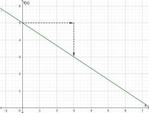
Graph [latex]f(x)=5-\frac{2}{3}x[/latex] using the vertical intercept and slope.
Answer:
In this function, [latex]x[/latex] is the input so it will be on the horizontal axis and [latex]f(x)[/latex] is the output so it will be on the vertical axis.
Since [latex]f(0)=5[/latex], the vertical intercept of the line is (0, 5).
In addition, the slope is [latex]-\frac{2}{3}=\frac{-2}{3}=\frac{\Delta\text{output}}{\Delta\text{input}}[/latex]. This tells us that for every increase by 3 units in input [latex]x[/latex], the output [latex]f[/latex] will decrease by 2 units.
In graphing, we can use this information by first plotting our vertical intercept on the graph, then using the slope to find a second point. From the initial value (0, 5) the slope tells us that if we move to the right 3, we will move down 2, moving us to the point (3, 3). We can continue this again to find a third point at (6, 1). Finally, extend the line to the left and right, containing these points.
Graphing Using Transformations
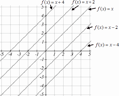
Another option for graphing is to use transformations of the identity function [latex]f(x)=x[/latex].
In the equation [latex]f(x)=mx[/latex], the [latex]m[/latex] is acting as the vertical stretch of the identity function. When [latex]m[/latex] is negative, there is also a vertical reflection of the graph. Looking at some examples will also help show the effect of slope on the shape of the graph:

In [latex]f(x)=mx+b[/latex], the [latex]b[/latex] acts as the vertical shift, moving the graph up and down without affecting the slope of the line. Some examples:
Example 8
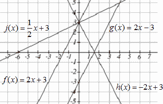
Match each equation with one of the lines in the graph below
[latex]\begin{align*} f(x) & = 2x+3\\ g(x) & = 2x-3\\ h(x) & = -2x+3\\ j(x) & = \frac{1}{2}x+3 \end{align*}[/latex]
Answer:
Only one graph has a vertical intercept of -3, so we can immediately match that graph with [latex]g(x)[/latex]. For the three graphs with a vertical intercept at 3, only one has a negative slope, so we can match that line with [latex]h(x)[/latex]. Of the other two, the steeper line would have a larger slope, so we can match that graph with equation [latex]f(x)[/latex], and the flatter line with the equation [latex]j(x)[/latex].
In addition to understanding the basic behavior of a linear function (increasing or decreasing, recognizing the slope and vertical intercept), it is often helpful to know the horizontal intercept of the function – where it crosses the horizontal axis.
Finding Horizontal Intercept
Example 9
Find the horizontal intercept of [latex]f(x)=-3+\frac{1}{2}x[/latex]
Answer:
Setting the function equal to zero to find what input will put us on the horizontal axis:
[latex]\begin{align*} 0 & = -3+\frac{1}{2}x\\ 3 & = \frac{1}{2}x\\ x & = 6 \end{align*}[/latex]
Thus the graph crosses the horizontal axis at [latex](6,0)[/latex].
Intersections of Lines
The graphs of two lines will intersect if they are not parallel. They will intersect at the point that satisfies both equations. To find this point when the equations are given as functions, we can solve for an input value so that [latex]f(x)=g(x)[/latex]. In other words, we can set the formulas for the lines equal, and solve for the input that satisfies the equation.
Economics tells us that in a free market, the price for an item is related to the quantity that producers will supply and the quantity that consumers will demand. Increases in prices will decrease demand, while supply tends to increase with prices. Sometimes supply and demand are modeled with linear functions.
Example 10
The supply, in thousands of items, for custom phone cases can be modeled by the equation [latex]s(p)=0.5+1.2p[/latex] while the demand can be modeled by [latex]d(p)=8.7-0.7p[/latex], where [latex]p[/latex] is in dollars. Find the equilibrium price and quantity, the intersection of the supply and demand curves.
Answer:
Setting [latex]s(p)=d(p)[/latex], we find
[latex]\begin{align*} 0.5+1.2p & = 8.7-0.7p\\ 1.9p & = 8.2\\ p & \approx \$4.32 \end{align*}[/latex]
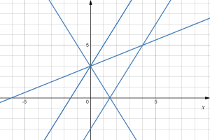
We can find the output value of the intersection point by evaluating either function at this input: [latex]s(4.32)=0.5+1.2(4.32)\approx 5.68[/latex]
These lines intersect at the point [latex](4.32, 5.68)[/latex]. If we graph the two functions we can verify that this result seems reasonable:
Business Applications
In business, a very common application of functions is to model cost, revenue, and profit.
Cost, Revenue, Profit
When a company produces [latex]x[/latex] items, the total cost [latex]C(x)[/latex] is the cost of total cost of producing those items. The total cost includes both fixed costs, which are startup costs, like equipment and buildings, and variable costs, which are costs that depend on the number of items produced, like materials and labor. In the most simple case, Cost = (variable cost rate)\cdot (number of units produced)+(fixed cost):
[latex]C(x)=c_{variable} \cdot x+c_{fixed}[/latex]
Revenue is the amount of money a company brings in from sales. In the most simple case, Revenue = (number of units sold)\cdot (price per unit):
[latex]R(x)=x\cdot p(x)[/latex]
Profit is the amount of money brings in, after expenses, i.e., Profit = Revenue – Cost:
[latex]P(x)=R(x)-C(x)[/latex]
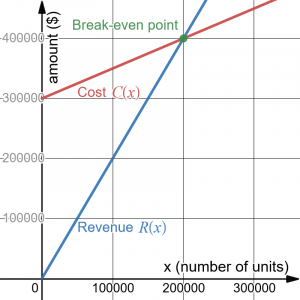
In marketing and financial planning, we often talk about the break-even point. This is the level of sales where the revenue equals the cost, or equivalently where profit is zero. This is typically the minimum level of sales necessary for the company to make a profit. The break-even point will occur when [latex]R(x)=C(x)[/latex] or, equivalently, when [latex]P(x)=0[/latex].
Example 11
A tech startup is looking at developing and launching a new mobile app. Initial development of the app will cost $300,000, and they estimate marketing and support for each user will cost $0.50. While the app will be free, they estimate they will be able to bring in $2 per user on average from in-app purchases. How many users will the company need to break even?
Answer:
We start by modeling the cost, revenue, and profit. Let [latex]x[/latex] = number of users.
The fixed (initial) costs are $300,000, and the variable (per-item) costs as $0.50 per user. We can write the total cost equation:
[latex]C(x)=300 000+0.50x[/latex]
The revenue will be $2 per user, so the revenue equation will be:
[latex]R(x) = 2x[/latex]
We could find the break-even point by setting the total cost equal to the revenue, which is equivalent to finding the intersection of the lines.
Algebraically: [latex]x=?, R(x)=C(x)[/latex]
[latex]R(x)=C(x)\Rightarrow 300000 + 0.50x=2x\Rightarrow 300000=1.5x\Rightarrow x=200000[/latex]
Therefore, the break-even point occurs at [latex]x=200000[/latex] users and the sales from in-app purchased in the amount of
[latex]R(200000)=2\cdot 200000=\$ 400,000[/latex].
Graphically:
Alternatively, we could go ahead and find a profit equation first:
[latex]P(x) = R(x) - C(x) = 2x - (300,000+0.50x) = 1.5x - 300,000[/latex]
The break even point can be found by setting the profit equal to zero:
[latex]\begin{align*} 0&=P(x)\\ &\Rightarrow 0 = 1.5x - 300,000\\ &\Rightarrow x = 200,000 \end{align*}[/latex]
The company will have to acquire 200,000 users to break-even.
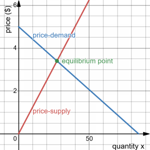
Supply and Demand
In economics, there is a model for how prices are determined in a free market which states that supply and demand for a product is related to the price. The demand relationship shows the quantity of a certain product that consumers are willing to buy at a certain price. Typically the quantity demanded will decrease for an item if the price increases. The supply relationship shows the quantity of a product that suppliers are willing to produce at a certain sales price. Typically the supply demanded will increase if the price increases. Economic theory says that supply and demand will interact, and the intersection will be the equilibrium price, or market price, where the quantity supplied and demanded will be equal.
Thus, we can think of the supply quantity and the demand quantity as functions of price.
If [latex]p[/latex] is the price of a product, then
[latex]x_D(p)[/latex] represents the quantity of the product that is demanded by the consumers at a given price [latex]p[/latex].
[latex]x_S(p)[/latex] represents the quantity of the product that is supplied by the producers at a given price [latex]p[/latex].
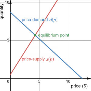
Since the demand for a product typically decreases as the price charged increases, the demand curve is typically a decreasing function.
Since the supply of a product typically increases as the price paid increases, the supply curve is typically an increasing function.
The intersection of the demand and the supply curves is the equilibrium price and quantity, also called the market price and quantity. This point is often denoted as [latex](\bar{p},\bar{x})[/latex].
Later in the course you will explore supply and demand curves that are non-linear, but in this section we will focus on linear supply and demand functions.
In most economic books you will see the supply and demand curve written with price as the input and quantity as the output, like [latex]x(p)[/latex]. However, supply and demand graphs are drawn with price on the vertical axis and quantity on the horizontal, in other words as a function [latex]p(x)[/latex]. Algebraically, we can write the equation in whichever way is more most appropriate for the context.
Example 12
At a price of $2.50 per gallon, there is a demand in a certain town for 42.5 thousand gallons of gas and a supply of 20 thousand gallons. At a price of $3.50, there is demand for 25.5 thousand gallons and a supply of 28 thousand gallons. Assuming supply and demand are linear, find the equilibrium price and quantity.
Answer:
We start by finding a linear equation for both supply and demand. We will use price, [latex]p[/latex] in dollars, as the output and quantity, [latex]x[/latex] in thousands of gallons, as the input.
For supply, we have the points [latex](20, 2.50)[/latex] and [latex](28, 3.50)[/latex].
Finding the slope: [latex]m = \dfrac{3.50-2.50}{28-20} = \frac{1}{8}[/latex]
We know the equation will look like [latex]p = \frac{1}{8}x+b[/latex], so substituting in [latex](20, 2.50)[/latex]
[latex]\begin{align*} 2.5 & = \frac{1}{8}(20) +b \\ 2.5 & = 2.5 +b \\ b & = 0 \end{align*}[/latex]
The supply equation is: [latex]p(x) = \frac{1}{8}x[/latex]$
For demand, we have the points [latex](42.5, 2.50)[/latex] and [latex](25.5, 3.50)[/latex].
Using a similar approach, we can find the demand equation is: [latex]p(x) = -\frac{1}{17}x+5[/latex]. (Verify.)
To find the equilibrium, we set the supply price equal to the demand price:
[latex]\frac{1}{8}x = -\frac{1}{17}x+5[/latex]
Multiplying through by 8(17) = 136 to clear the fractions,
[latex]136\left(\frac{1}{8}x\right) = 136\left(-\frac{1}{17}x+5\right)[/latex]
[latex]17x = -8x+680[/latex]
Now we solve for [latex]x[/latex].
[latex]25x = 680[/latex]
[latex]x = 27.2[/latex], which is the equilibrium quantity.
To find the equilibrium price, we can substitute the equilibrium quantity back into either equation:
[latex]p = \frac{1}{8}(27.2) = 3.4[/latex]
The equilibrium will be achieved at [latex]\bar{x}=27.2[/latex] thousand gallons of gas at a price of [latex]\bar{p}=\$3.40[/latex].
Graphically:
Concept in Action – Modeling Using Data
Complete the following set of exercises that will put into practice many of the concepts discussed in this section.
Mathmatize: Price, supply and demand investigation
Section Exercises – after the reading
Work on section 8.2 exercises in Fundamentals of Business Math Exercises after reading this section. Discuss your solutions with your peers and/or course instructor.
You may consult answers to select exercises: Fundamentals of Business Math Exercises – Select Answers
