8.5 Polynomial and Rational Functions
Polynomial Functions
Terminology of Polynomial Functions
Each of the [latex]a_i[/latex] constants are called coefficients and can be positive, negative, or zero, and be whole numbers, decimals, or fractions.
A term of the polynomial is any one piece of the sum, that is any [latex]a_i x^i[/latex]. Each individual term is a transformed power function.
The degree of the polynomial is the highest power of the variable that occurs in the polynomial.
The leading term is the term containing the highest power of the variable: the term with the highest degree.
The leading coefficient is the coefficient of the leading term.
Because of the definition of the “leading” term we often rearrange polynomials so that the powers are descending: [latex]f(x)=a_n x^n+a_{n-1}x^{n-1}\dots a_2 x^2+a_1 x+a_0[/latex]
Example 1
Answer: The degree is 3, the highest power on [latex]x[/latex]. The leading term is the term containing that power, [latex]-4x^3[/latex]. The leading coefficient is the coefficient of that term, -4.
Intercepts
As with any function, the vertical intercept can be found by evaluating the function at an input of zero. Since this is evaluation, it is relatively easy to do it for a polynomial of any degree – it will always be equal to the value of the constant term.
On the other hand, to find horizontal intercepts, we need to solve for when the output will be zero. For general polynomials, this can be a challenging prospect. Consequently, we will limit ourselves to three cases:
- The polynomial can be factored using known methods: greatest common factor, difference of squares, and quadratic formula.
- The polynomial is given in factored form.
- Technology is used to determine the intercepts.
Recall the difference of squares formula:
[latex]a^2-b^2=(a-b)(a+b)[/latex]
Recall the factoring of a quadratic using the quadratic formula:
[latex]ax^2+bx+c=a(x-x_1)(x-x_2)\text{ where } x_{1,2}=\frac{-b\pm\sqrt{b^2-4ac}}{2a}[/latex]
Example 2
Find the horizontal intercepts of [latex]f(x)=x^6-3x^4+2x^2[/latex].
Answer:
We can attempt to factor this polynomial to find solutions for [latex]f(x) = 0[/latex]:
[latex]x^6-3x^4+2x^2=0\rightarrow[/latex] factoring out the greatest common factor:
[latex]x^2(x^4-3x^2+2)=0\rightarrow[/latex] factoring the expression in the bracket as a quadratic in variable [latex]yx^2[/latex]:
[latex]\begin{align*} x^4-3x^2+2&=y^2-3y+2=a(y-y_1)(y-y_2)\\ &\Rightarrow y_{1,2}=\frac{-(-3)\pm\sqrt{(-3)^2-4\cdot 1\cdot 2}}{2\cdot 1}=\frac{3\pm 1}{2}\\ &\Rightarrow y_1=2, y_2=1\\ &\Rightarrow x^4-3x^2+2=1\cdot(x^2-2)(x^2-1)\\ &\Rightarrow x^4-3x^2+2=(x-\sqrt{2})(x+\sqrt{2})(x-1)(x+1) \end{align*}[/latex]
And so
[latex]x^2(x-\sqrt{2})(x+\sqrt{2})(x-1)(x+1)=0[/latex] if and only if [latex]x=0, \sqrt{2}, -\sqrt{2}, 1[/latex] or [latex]-1[/latex].
This gives us five horizontal intercepts: [latex](0,0),(\sqrt{2},0), ( -\sqrt{2},0), (1,0)[/latex] and [latex](-1,0)[/latex].
Example 3
Find the horizontal intercepts of [latex]h(t)=t^3+4t^2+t-6[/latex]
Answer:
Since this polynomial is not in factored form, has no common factors, and does not appear to be factorable using techniques we know, we can turn to technology to find the intercepts.
Graphing this function using an online calculator (for example, see its graph on Desmos), it appears there are horizontal intercepts at [latex]t = -3, -2,[/latex] and [latex]1[/latex].
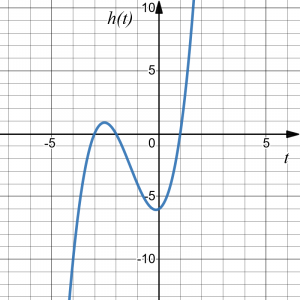
We could check these are correct by plugging in these values for [latex]t[/latex] and verifying that, indeed, [latex]h(-3)=h(-2)=h(1)=0[/latex].
Solving Polynomial Inequalities
One application of our ability to find intercepts and sketch a graph of polynomials is the ability to solve polynomial inequalities. It is a very common question to ask when a function will be positive and negative, and one we will use later in this course.
Example 4
Solve [latex](x+3)(x+1)^2(x-4)\gt 0[/latex]
Answer:
As with all inequalities, we start by solving the equality [latex](x+3)(x+1)^2(x-4)= 0[/latex], which has solutions at [latex]x =[/latex] -3, -1, and 4. We know the function can only change from positive to negative at these values, so these divide the inputs into 4 intervals.
We can then choose a test value in each interval and evaluate each of the factors of the function [latex]f(x)=(x+3)(x+1)^2(x-4)[/latex] at each test value to determine if each of the factors, and thus the overall function, is positive or negative in that interval:
| Interval | [latex](-\infty,-3)[/latex] | [latex](-3,-1)[/latex] | [latex](-1,4)[/latex] | [latex](4,\infty)[/latex] |
| [latex](x+3)[/latex] | [latex]-[/latex] | [latex]+[/latex] | [latex]+[/latex] | [latex]+[/latex] |
| [latex](x+1)^2[/latex] | [latex]+[/latex] | [latex]+[/latex] | [latex]+[/latex] | [latex]+[/latex] |
| [latex](x-4)[/latex] | [latex]-[/latex] | [latex]-[/latex] | [latex]-[/latex] | [latex]+[/latex] |
| [latex](x+3)(x+1)^2(x-4)[/latex] | [latex]+[/latex] | [latex]-[/latex] | [latex]-[/latex] | [latex]+[/latex] |
Hence, [latex](x+3)(x+1)^2(x-4)\gt 0[/latex] on [latex](-\infty,-3)\cup (4,\infty)[/latex].
You can also verify this by defining a function [latex]f(x)=(x+3)(x+1)^2(x-4)[/latex] and graphing it using an graphing calculator such as Desmos. If we consider the graph of [latex]f(x)[/latex] (see Desmos), we can see that this function is positive, i.e., [latex]f(x)>0[/latex] on the intervals [latex](-\infty,-3)[/latex] and [latex](4,\infty)[/latex].
Rational Functions
Rational functions are the ratios, or fractions, of polynomials. They can arise from both simple and complex situations.
Example 5
Answer: You may recall that multiplying speed by time will give you distance. If we let [latex]t[/latex] represent the drive time in hours, and [latex]v[/latex] represent the velocity (speed or rate) at which we drive, then [latex]vt=[/latex] distance. Since our distance is fixed at 100 miles, [latex]vt=100[/latex]. Solving this relationship for the time gives us the function we desired: [latex]t(v)=\frac{100}{v}[/latex]
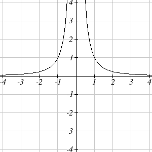
Notice that this is a transformation of the reciprocal toolkit function, [latex]f(x)=\dfrac{1}{x}[/latex]. Several natural phenomena, such as gravitational force and volume of sound, behave in a manner inversely proportional to the square of another quantity. For example, the volume, [latex]V[/latex], of a sound heard at a distance [latex]d[/latex] from the source would be related by [latex]V=\dfrac{k}{d^2}[/latex] for some constant value [latex]k[/latex]. These functions are transformations of the reciprocal squared toolkit function [latex]f(x)=\dfrac{1}{x^2}[/latex].
In business the most common rational function is the average cost function [latex]\bar{C}(x)[/latex]:
[latex]\bar{C}(x)=\frac{C(x)}{x}, \ \ \ \ x>0[/latex]
where [latex]x[/latex] is the number of units and [latex]C(x)[/latex] is the cost of producing [latex]x[/latex] units. Then [latex]\bar{C}(x)[/latex] represents the average cost per unit if [latex]x[/latex] units are produced.
We have seen the graphs of the basic reciprocal function and the squared reciprocal function from our review of toolkit functions. These graphs have several important features.
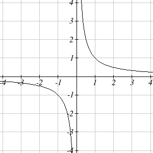
Let’s begin by looking at the reciprocal function, [latex]f(x)=\dfrac{1}{x}[/latex]. As you well know, dividing by zero is not allowed and therefore zero is not in the domain, and so the function is undefined at an input of zero.
Short Run behavior:
As the input values approach zero from the left side (taking on very small, negative values), the function values become very large in the negative direction (in other words, they approach negative infinity). We write: [latex]x\to 0^-[/latex], [latex]f(x)\to -\infty[/latex].
As we approach zero from the right side (small, positive input values), the function values become very large in the positive direction (approaching infinity). We write: as [latex]x\to 0^+[/latex], [latex]f(x)\to \infty[/latex].
This behavior creates a vertical asymptote.
An asymptote is a line that the graph approaches. In this case the graph is approaching the vertical line [latex]x = 0[/latex] as the input approaches zero.
Long Run behavior:
As the values of [latex]x[/latex] approach infinity, the function values approach 0. Also, as the values of [latex]x[/latex] approach negative infinity, the function values approach 0. Symbolically: as [latex]x\to\pm\infty[/latex], [latex]f(x)\to 0[/latex].
Based on this long run behavior and the graph we can see that the function approaches 0 but never actually reaches 0, it just “levels off” as the inputs become large. This behavior creates a horizontal asymptote . In this case the graph is approaching the horizontal line [latex]f(x)=0[/latex] as the input becomes very large in the negative and positive directions.
Vertical and Horizontal Asymptotes
A vertical asymptote of a graph is a vertical line [latex]x = a[/latex] where the graph tends towards positive or negative infinity as the inputs approach [latex]a[/latex]. As [latex]x\to a[/latex], [latex]f(x)\to\pm\infty[/latex].
A horizontal asymptote of a graph is a horizontal line [latex]y=b[/latex] where the graph approaches the line as the inputs get large. As [latex]x\to\pm\infty[/latex], [latex]f(x)\to b[/latex].
Example 6
Sketch a graph of the reciprocal function shifted two units to the left and up three units. Identify the horizontal and vertical asymptotes of the graph, if any.
Answer:
Transforming the graph left 2 and up 3 would result in the function [latex]f(x)=\dfrac{1}{x+2}+3[/latex], or equivalently, by giving the terms a common denominator, [latex]f(x)=\dfrac{3x+7}{x+2}.[/latex]
Shifting the toolkit function would give us this graph. Notice that this equation is undefined at [latex]x = -2[/latex], and the graph also is showing a vertical asymptote at [latex]x = -2[/latex]. As [latex]x\to -2^-[/latex], [latex]f(x)\to -\infty[/latex], and as [latex]x\to -2^+[/latex], [latex]f(x)\to \infty[/latex].
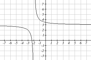
As the inputs grow large, the graph appears to be leveling off at output values of 3, indicating a horizontal asymptote at [latex]y=3[/latex]. As [latex]x\to\pm\infty[/latex], [latex]f(x)\to 3[/latex]
Notice that horizontal and vertical asymptotes get shifted left 2 and up 3 along with the function.
A general rational function is the ratio of any two polynomials.
[latex]f(x)=\frac{P(x)}{Q(x)}=\frac{a_0+a_1 x+a_2 x^2+\dots+a_p x^p}{b_0+b_1 x+b_2 x^2+\dots+b_q x^q}[/latex]
Rational functions can arise from real situations.
Example 7
Answer:
Notice that the amount of water in the tank is changing linearly, as is the amount of sugar in the tank. We can write an equation independently for each:[latex]\text{water}=100+10t \qquad \text{sugar}=5+1t[/latex]
The concentration, [latex]C[/latex], will be the ratio of pounds of sugar to gallons of water: [latex]C(t)=\frac{5+t}{100+10t}[/latex]
Domain, Holes and Vertical Asymptotes of a Rational Function
The domain of a rational function will be all real numbers except for those that make the denominator zero.
The vertical asymptotes of a rational function will occur where the denominator of the function is equal to zero and the numerator is not zero.
If both the numerator and the denominator are zero for some input value, then the graph of the function has a hole at that input value.
Typically, to determine whether and where a rational function has a vertical asymptote and/or a hole, we must rewrite both the numerator and the denominator in the factored form, and use that to determine for which input values each of them is zero.
For example, the function [latex]f(x)=\dfrac{5x^2-14x-3}{2x^2-6x}[/latex] can be factored using quadratic formula as follows (verify):
[latex]f(x)=\frac{5\left(x+\dfrac{1}{5}\right)(x-3)}{2x(x-3)}[/latex]
Numerator [latex]= 0: x=\frac{1}{5}, 3[/latex]
Denominator [latex]=0: x=0, 3[/latex]
Therefore, there is a vertical asymptote at [latex]x=0[/latex] and a hole at [latex]x=3[/latex].
Graphically: Desmos
Horizontal Asymptote of a Rational Function
The horizontal asymptote of a rational function can be determined by looking at the degrees of the numerator and denominator. Suppose we have:
[latex]f(x)=\frac{a_mx^m+a_{m-1}x^{m-1}+\ldots+a_1x+a_0}{b_nx^n+b_{n-1}x^{n-1}+\ldots+b_1x+b_0}[/latex]
- Degree of denominator > degree of numerator: horizontal asymptote at [latex]y=0[/latex].
- Degree of denominator < degree of numerator: no horizontal asymptote.
- Degree of denominator = degree of numerator: horizontal asymptote at ratio of leading coefficients, [latex]y=\dfrac{a_m}{b_n}[/latex] ([latex]m[/latex] and [latex]n[/latex] are equal in this case).
In business, you can think of the horizontal asymptote as a “floor” or a “ceiling”, depending on how the graph of the function behaves around the asymptote.
Example 8
In the sugar concentration problem from earlier, we created the equation [latex]C(t)=\frac{5+t}{100+10t}[/latex]. Find the horizontal asymptote and interpret it in context of the scenario.
Answer:
Both the numerator and denominator are linear (degree 1), so since the degrees are equal, there will be a horizontal asymptote at the ratio of the leading coefficients. In the numerator, the leading term is [latex]t[/latex], with coefficient 1. In the denominator, the leading term is [latex]10t[/latex], with coefficient 10. The horizontal asymptote will be at the ratio of these values: As [latex]t \to \infty[/latex], [latex]C(t)\to \frac{1}{10}[/latex]. This function will have a horizontal asymptote at [latex]y=\frac{1}{10}[/latex].
This tells us that as the input gets large, the output values will approach [latex]\frac{1}{10}[/latex]. In context, this means that as more time goes by, the concentration of sugar in the tank will approach one tenth of a pound of sugar per gallon of water or [latex]\frac{1}{10}[/latex] pounds per gallon.
Example 9
Answer: First, note this function is has no inputs that make both the numerator and denominator zero, so there are no potential holes. The function will have vertical asymptotes when the denominator is zero, causing the function to be undefined. The denominator will be zero at [latex]x =[/latex] 1, -2, and 5, indicating vertical asymptotes at these values.
The numerator has degree 2, while the denominator has degree 3. Since the degree of the denominator is greater than the degree of the numerator, the denominator will grow faster than the numerator, causing the outputs to tend towards zero as the inputs get large, and so as [latex]x\to\pm\infty[/latex], [latex]f(x)\to 0[/latex]. This function will have a horizontal asymptote at [latex]y=0[/latex].
Example 10
A manufacturer has determined that it costs them $68,220 to produce 7,000 units of a specific product per day and $81,000 to produce 9,000 per day. Assuming that the cost and the production are linearly related, determine the cost function [latex]C(x)[/latex] and the average cost function [latex]\bar{C}(x)[/latex] in terms of the daily production of [latex]x[/latex] number of units. Determine their domains and holes, vertical asymptotes and horizontal asymptotes, if any, and interpret their meaning in the context of this problem. Calculate [latex]C(20000)[/latex]and [latex]\bar{C}(20000)[/latex] and interpret the results.
Answer:
Task: [latex]C(x)=?[/latex], [latex]\bar{C}(x)=?[/latex] where [latex]C[/latex] is cost, [latex]\bar{C}[/latex] is average daily cost, [latex]x[/latex] is number of units produced per day; domain, holes and asymptotes and interpretation for each?; [latex]C(20000)=?[/latex] , [latex]\bar{C}(2000)=?[/latex], interpretation for each?
Conditions: [latex]C[/latex] and [latex]x[/latex] linearly related [latex]\Rightarrow C(x)=mx+b[/latex] for some [latex]m[/latex] and [latex]b[/latex].
[latex]C(x)=?[/latex]
[latex]m=\frac{\text{change in output}}{\text{change in input}}=\frac{68220 -81000}{7000-9000}=6.39[/latex]
Therefore, [latex]C(x)=6.39x+b[/latex].
[latex]b=?:[/latex] at [latex]x=7000, C(x)=68220[/latex] and so
[latex]\begin{align*} 68220=6.39(7000)+b&\Rightarrow b=68220-6.39(7000)=23490\\ &\Rightarrow C(x)=6.39x+23490 \end{align*}[/latex]
domain of [latex]C(x)[/latex]?
[latex]C(x)[/latex] can be calculated for all [latex]x[/latex], but [latex]x=[/latex] number of units, so [latex]x\ge 0[/latex].
Therefore, domain of [latex]C(x)[/latex]: [latex][0,\infty)[/latex], i.e., theoretically, the cost can be calculated using [latex]C(x)=6.39x+23490[/latex] for any nonnegative value of [latex]x[/latex].
holes, vertical asymptotes of [latex]C(x)[/latex]?
[latex]C(x)[/latex] is a linear function, so it is a polynomial, and therefore has no holes or vertical or horizontal asymptotes.
[latex]\bar{C}(x)=?[/latex]
[latex]\bar{C}(x)=\frac{C(x)}{x}=\frac{6.39x+23490}{x}=6.39+\frac{23490}{x}[/latex]
domain of [latex]\bar{C}(x)[/latex]?
[latex]\bar{C}(x)[/latex] can be calculated for all [latex]x\neq 0[/latex], but [latex]x=[/latex] number of units, so [latex]x> 0[/latex].
Therefore, domain of [latex]\bar{C}(x)[/latex]: [latex](0,\infty)[/latex].
Note that this makes sense because we can’t calculate average cost if no units have been produced, i.e., if [latex]x=0[/latex].
holes, vertical asymptotes of [latex]\bar{C}(x)[/latex]?
[latex]\bar{C}(x)[/latex] is a rational function, so we must investigate when the denominator is zero and check that against when the numerator is zero.
Since the denominator is zero only when [latex]x=0[/latex] and the numerator is not equal to zero when [latex]x=0[/latex], we get a vertical asymptote at [latex]x=0[/latex], with [latex]\bar{C}(x)=6.39+\frac{23490}{x}[/latex] approaching [latex]\infty[/latex]. In other words, the average cost per unit approaches infinity as the number of units approaches 0.
Since the numerator and the denominator are of the same degree (1, since linear), there will be a horizontal asymptote at [latex]\frac{6.39}{1}=6.39[/latex]. This means that in the long run, as the production increases, the average cost approaches the value of $6.39/unit.
Note that this makes sense in the business context because, when calculating the average cost per unit, the fixed cost is spread out across the units. So the more units are produced, the less of a contribution the fixed cost makes to the average cost of one unit. This makes the average cost very close to the variable cost per unit if the daily production gets sufficiently high. You can also visualize that from [latex]\bar{C}(x)=6.39+\frac{23490}{x}[/latex] because, as [latex]x[/latex] approaches infinity, the value of [latex]\frac{23490}{x}[/latex] approaches 0.
[latex]C(20000)=?[/latex]
[latex]C(2000)=6.39(20000)+23490=151290[/latex]
This means that the cost of producing 20,000 units per day is $151,290.
[latex]\bar{C}(20000)=?[/latex]
[latex]\bar{C}(20000)=6.39+\frac{23490}{20000}=7.5645 \approx 7.56[/latex]
This means that, at the daily production level of 20,000 units, the average cost is approximately $7.56 per unit.
For visualization, here are the graphs of the cost function [latex]C(x)[/latex] and the average cost function [latex]\bar{C}(x)[/latex]. Confirm visually their characteristics that we determined above.
Cost function: Desmos
Average cost function: Desmos
Horizontal and Vertical Intercepts of a Rational Function
As with all functions, a rational function will have a vertical intercept when the input is zero, if the function is defined at zero. It is possible for a rational function to not have a vertical intercept if the function is undefined at zero. This will occur when the numerator is zero, but the denominator is not.
Likewise, a rational function will have horizontal intercepts at the inputs that cause the output to be zero (unless that input corresponds to a hole). It is possible there are no horizontal intercepts. Since a fraction is only equal to zero when we are dividing zero with a non-zero number, horizontal intercepts will occur when the numerator of the rational function is equal to zero but the denominator is not.
Example 11
Answer: We can find the vertical intercept by evaluating the function at zero: [latex]f(0)=\frac{(0-2)(0+3)}{(0-1)(0+2)(0-5)}=\frac{-6}{10}=-\frac{3}{5}.[/latex]
The horizontal intercepts will occur when the function is equal to zero:
[latex]\begin{align*} 0 & = \frac{(x-2)(x+3)}{(x-1)(x+2)(x-5)} \qquad \text{(This is zero when the numerator is zero.)}\\ &\\ &\Rightarrow 0 = (x-2)(x+3)\\ &\\ &\Rightarrow x = 2, -3 \end{align*}[/latex]
Summary of characteristics of polynomial and rational functions
Summary of characteristics of polynomial functions
A polynomial function is defined on all real numbers, i.e., its domain is [latex](-\inft,\infty)[/latex].
A polynomial function has no holes or asymptotes.
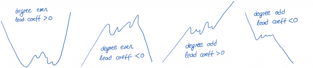
A polynomial function approaches [latex]\infty[/latex] or [latex]-\infty[/latex] in the long run, depending on the degree and the leading coefficient of the polynomial.
The vertical intercept of a polynomial function is the value of its constant term.
The horizontal intercepts of a polynomial function are the zeros of the factors of the polynomial. If [latex]n[/latex] is the degree of the polynomial, the polynomial has at most [latex]n[/latex] horizontal intercepts, i.e., zeros.
Summary of characteristics of rational functions
A rational function is defined on all real numbers except those that make the denominator 0, if any.
A rational function may have holes or vertical or horizontal asymptotes (or it may have none of them).
To determine whether a rational function has holes or vertical asymptotes, we must analyze the zeros of the numerator and the denominator.
- Factor the numerator and the denominator fully.
- If there are factors in the numerator and the denominator that can be equal to 0 for some input value and the factors cancel out fully, then there is a hole in the graph of the function at that input value.
- If there are factors in the numerator and the denominator that can be equal to 0 for some input value but do not cancel out fully, then there is a vertical asymptote in the graph of the function at that input value.
To determine whether a rational function has a horizontal asymptote, we must analyze the degrees and the leading coefficients of both the numerator and the denominator.
- If the degrees of the numerator and the denominator are equal, there is a horizontal asymptote at output value equal to the fraction
[latex]\frac{\text{ leading coefficient of the numerator}}{\text{ leading coefficient of the denominator}}[/latex] - If the degree of the numerator is smaller than the degree of the denominator, there is a horizontal asymptote at output value of 0, i.e., the horizontal axis is the horizontal asymptote.
- If the degree of the numerator is larger than the degree of the denominator, there is no horizontal asymptote.
The vertical intercept of a rational function, if any, is the value of the function at the input value 0.
The horizontal intercepts of a rational function are the zeros of the factors of the numerator that are not also zeros of the factors of the denominator. If [latex]n[/latex] is the degree of the numerator, the function has at most [latex]n[/latex] horizontal intercepts, i.e., zeros.
