3.8 Chapter 3 Example Solutions

Example 1: Adding a Constant to a Function

We can sketch a graph of this new function by adding 20 to each of the output values of the original function. This will have the effect of shifting the graph vertically up, as shown in Figure 3-21.

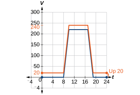
Notice that in Figure 3-21, for each input value, the output value has increased by 20, so if we call the new function [latex]\text{}S\left(t\right)[/latex], we could write

[latex]S\left(t\right)=V\left(t\right)+20[/latex]

This notation tells us that, for any value of [latex]\text{}t,S\left(t\right)\text{}[/latex] can be found by evaluating the function [latex]\text{}V\text{}[/latex] at the same input and then adding 20 to the result. This defines [latex]\text{}S\text{}[/latex] as a transformation of the function [latex]\text{}V\text{}[/latex], in this case a vertical shift up 20 units. Notice that, with a vertical shift, the input values stay the same and only the output values change. See Table 8.

Table 8

[latex]t[/latex]	0	8	10	17	19	24
[latex]V\left(t\right)[/latex]	0	0	220	220	0	0
[latex]S\left(t\right)[/latex]	20	20	240	240	20	20

Example 2: Shifting a Tabular Function Vertically

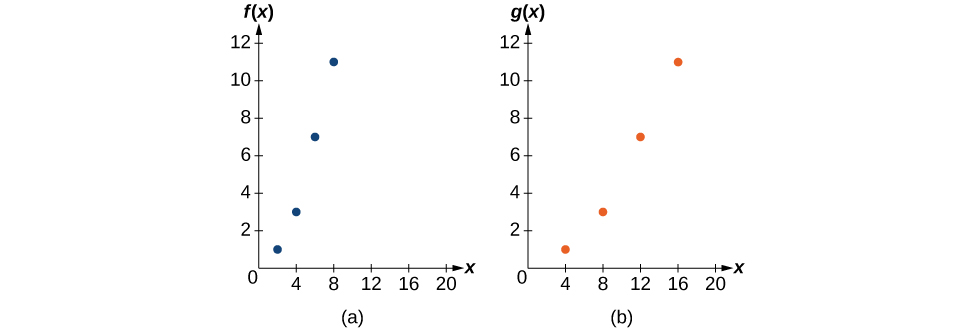
The formula [latex]\text{}g\left(x\right)=f\left(x\right)-3\text{}[/latex] tells us that we can find the output values of [latex]\text{}g\text{}[/latex] by subtracting 3 from the output values of [latex]\text{}f\text{}[/latex]. For example:

[latex]\begin{array}{ll}f\left(2\right)=1\hfill & \text{Given}\hfill \\ g\left(x\right)=f\left(x\right)-3\hfill & \text{Given transformation}\hfill \\ g\left(2\right)=f\left(2\right)-3\hfill & \hfill \\ \text{}\text{}\text{}\text{}\text{}\text{}\text{}\text{}\text{}\text{}=1-3\hfill & \hfill \\ \text{}\text{}\text{}\text{}\text{}\text{}\text{}\text{}\text{}\text{}=-2\hfill & \hfill \end{array}[/latex]

Subtracting 3 from each [latex]\text{}f\left(x\right)\text{}[/latex] value, we can complete a table of values for [latex]\text{}g\left(x\right)\text{}[/latex] as shown in Table 9.

Table 9

[latex]x[/latex]	2	4	6	8
[latex]f\left(x\right)[/latex]	1	3	7	11
[latex]g\left(x\right)[/latex]	−2	0	4	8

Example 3: Vertical Shift

[latex]b\left(t\right)=h\left(t\right)+10=-4.9{t}^{2}+30t+10[/latex]

Example 4: Adding a Constant to an Input

We can set [latex]\text{}V\left(t\right)\text{}[/latex] to be the original program and [latex]\text{}F\left(t\right)\text{}[/latex] to be the revised program.

[latex]\begin{array}{c}\text{}\text{}\text{}\text{}\text{}\text{}\text{}\text{}\text{}\text{}\text{}\text{}\text{}V\left(t\right)=\text{ the original venting plan}\\ \text{F}\left(t\right)=\text{starting 2 hrs sooner}\end{array}[/latex]

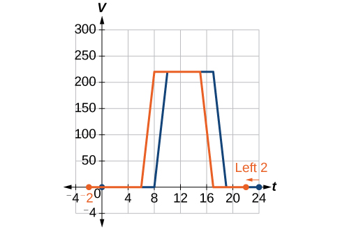
In the new graph, at each time, the airflow is the same as the original function [latex]\text{}V\text{}[/latex] was 2 hours later. For example, in the original function [latex]\text{}V,\text{}[/latex] the airflow starts to change at 8 a.m., whereas for the function [latex]\text{}F,\text{}[/latex] the airflow starts to change at 6 a.m. The comparable function values are [latex]\text{}V\left(8\right)=F\left(6\right)\text{}[/latex]. See Figure 3-22. Notice also that the vents first opened to [latex]\text{}220{\text{ ft}}^{2}\text{}[/latex] at 10 a.m. under the original plan, while under the new plan the vents reach [latex]\text{}220{\text{ ft}}^{\text{2}}\text{}[/latex] at 8 a.m., so [latex]\text{}V\left(10\right)=F\left(8\right)[/latex].

In both cases, we see that, because [latex]\text{}F\left(t\right)\text{}[/latex] starts 2 hours sooner, [latex]\text{}h=-2\text{}[/latex]. That means that the same output values are reached when [latex]\text{}F\left(t\right)=V\left(t-\left(-2\right)\right)=V\left(t+2\right)[/latex].

Example 5: Shifting a Tabular Function Horizontally

The formula [latex]\text{}g\left(x\right)=f\left(x-3\right)\text{}[/latex] tells us that the output values of [latex]\text{}g\text{}[/latex] are the same as the output value of [latex]\text{}f\text{}[/latex] when the input value is 3 less than the original value. For example, we know that [latex]\text{}f\left(2\right)=1\text{}[/latex]. To get the same output from the function [latex]\text{}g\text{}[/latex], we will need an input value that is 3 larger. We input a value that is 3 larger for [latex]\text{}g\left(x\right)\text{}[/latex] because the function takes 3 away before evaluating the function [latex]\text{}f[/latex].

[latex]\begin{array}{l}g\left(5\right)=f\left(5-3\right)\hfill \\ \text{}\text{}\text{}\text{}\text{}\text{}\text{}\text{}\text{}\text{}\text{}=f\left(2\right)\hfill \\ \text{}\text{}\text{}\text{}\text{}\text{}\text{}\text{}\text{}\text{}\text{}=1\hfill \end{array}[/latex]

We continue with the other values to create Table 9.

Table 9

[latex]x[/latex]	5	7	9	11
[latex]x-3[/latex]	2	4	6	8
[latex]f\left(x-3\right)[/latex]	1	3	7	11
[latex]g\left(x\right)[/latex]	1	3	7	11

The result is that the function [latex]\text{}g\left(x\right)\text{}[/latex] has been shifted to the right by 3. Notice the output values for [latex]\text{}g\left(x\right)\text{}[/latex] remain the same as the output values for [latex]\text{}f\left(x\right)\text{}[/latex], but the corresponding input values, [latex]\text{}x\text{}[/latex], have shifted to the right by 3. Specifically, 2 shifted to 5, 4 shifted to 7, 6 shifted to 9, and 8 shifted to 11.

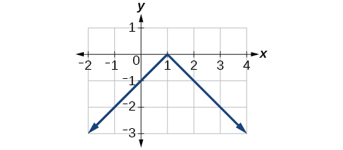
Example 6: Identifying a Horizontal Shift of a Toolkit Function

Notice that the graph is identical in shape to the [latex]\text{}f\left(x\right)={x}^{2}\text{}[/latex] function, but the x-values are shifted to the right 2 units. The vertex used to be at (0,0), but now the vertex is at (2,0). The graph is the basic quadratic function shifted 2 units to the right, so

[latex]g\left(x\right)=f\left(x-2\right)[/latex]

Notice how we must input the value [latex]\text{}x=2\text{}[/latex] to get the output value [latex]\text{}y=0\text{}[/latex]; the x-values must be 2 units larger because of the shift to the right by 2 units. We can then use the definition of the [latex]\text{}f\left(x\right)\text{}[/latex] function to write a formula for [latex]\text{}g\left(x\right)\text{}[/latex] by evaluating [latex]\text{}f\left(x-2\right)[/latex].

[latex]\begin{array}{l}f\left(x\right)={x}^{2}\hfill \\ g\left(x\right)=f\left(x-2\right)\hfill \\ g\left(x\right)=f\left(x-2\right)={\left(x-2\right)}^{2}\hfill \end{array}[/latex]

Example 7: Interpreting Horizontal versus Vertical Shifts

1. [latex]G\left(m\right)+10\text{}[/latex] can be interpreted as adding 10 to the output, gallons. This is the gas required to drive [latex]\text{}m\text{}[/latex] miles, plus another 10 gallons of gas. The graph would indicate a vertical shift.

[latex]G\left(m+10\right)\text{}[/latex] can be interpreted as adding 10 to the input, miles. So this is the number of gallons of gas required to drive 10 miles more than [latex]\text{}m\text{}[/latex] miles. The graph would indicate a horizontal shift.

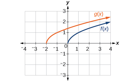
2. The graphs of [latex]\text{}f\left(x\right)\text{}[/latex] and [latex]\text{}g\left(x\right)\text{}[/latex] are shown below. The transformation is a horizontal shift. The function is shifted to the left by 2 units.

Example 8: Graphing Combined Vertical and Horizontal Shifts

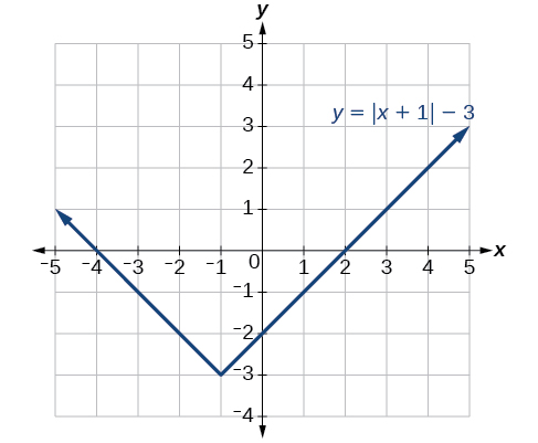
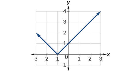
1. The function [latex]\text{}f\text{}[/latex] is our toolkit absolute value function. We know that this graph has a V shape, with the point at the origin. The graph of [latex]\text{}h\text{}[/latex] has transformed [latex]\text{}f\text{}[/latex] in two ways: [latex]\text{}f\left(x+1\right)\text{}[/latex] is a change on the inside of the function, giving a horizontal shift left by 1, and the subtraction by 3 in [latex]\text{}f\left(x+1\right)-3\text{}[/latex] is a change to the outside of the function, giving a vertical shift down by 3. The transformation of the graph is illustrated in Figure 3-23.

Let us follow one point of the graph of [latex]\text{}f\left(x\right)=|x|[/latex].

• The point [latex]\left(0,0\right)[/latex] is transformed first by shifting left 1 unit: [latex]\left(0,0\right)\to \left(-1,0\right)[/latex]
• The point [latex]\left(-1,0\right)[/latex] is transformed next by shifting down 3 units: [latex]\left(-1,0\right)\to \left(-1,-3\right)[/latex]

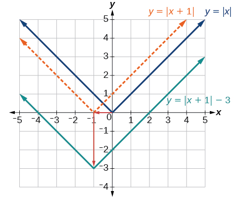
Figure 3-24 shows the graph of [latex]\text{}h[/latex].

2.

Example 9: Identifying Combined Vertical and Horizontal Shifts

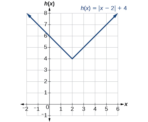
1. The graph of the toolkit function starts at the origin, so this graph has been shifted 1 to the right and up 2. In function notation, we could write that as

[latex]h\left(x\right)=f\left(x-1\right)+2[/latex]

Using the formula for the square root function, we can write

[latex]h\left(x\right)=\sqrt{x-1}+2[/latex]

2. [latex]g\left(x\right)=\frac{1}{x-1}+1[/latex]

Example 1: Reflecting a Graph Horizontally and Vertically

1. a. Reflecting the graph vertically means that each output value will be reflected over the horizontal t-axis as shown in Figure 3-25.

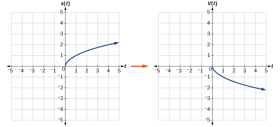
Because each output value is the opposite of the original output value, we can write

[latex]V\left(t\right)=-s\left(t\right)\text{ or }V\left(t\right)=-\sqrt{t}[/latex]

Notice that this is an outside change, or vertical shift, that affects the output [latex]\text{}s\left(t\right)\text{}[/latex] values, so the negative sign belongs outside of the function.

b. Reflecting horizontally means that each input value will be reflected over the vertical axis as shown in 3-26.

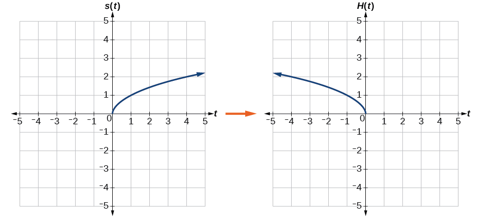
Because each input value is the opposite of the original input value, we can write

[latex]H\left(t\right)=s\left(-t\right)\text{ or }H\left(t\right)=\sqrt{-t}[/latex]

Notice that this is an inside change or horizontal change that affects the input values, so the negative sign is on the inside of the function.

Note that these transformations can affect the domain and range of the functions. While the original square root function has domain [latex]\text{}\left[0,\infty \right)\text{}[/latex] and range [latex]\text{}\left[0,\infty \right)\text{}[/latex], the vertical reflection gives the [latex]\text{}V\left(t\right)\text{}[/latex] function the range [latex]\left(-\infty ,\text{}0\right][/latex] and the horizontal reflection gives the [latex]\text{}H\left(t\right)\text{}[/latex] function the domain [latex]\left(-\infty ,\text{}0\right][/latex].

2.

1. 
2. 

Example 2: Reflecting a Tabular Function Horizontally and Vertically

1. a. For [latex]\text{}g\left(x\right)\text{}[/latex] the negative sign outside the function indicates a vertical reflection, so the x-values stay the same and each output value will be the opposite of the original output value. See Table 10.

Table 10

[latex]x[/latex]	2	4	6	8
[latex]\text{}g\left(x\right)\text{}[/latex]	–1	–3	–7	–11

b. For [latex]\text{}h\left(x\right)\text{}[/latex], the negative sign inside the function indicates a horizontal reflection, so each input value will be the opposite of the original input value and the [latex]\text{}h\left(x\right)\text{}[/latex] values stay the same as the [latex]\text{}f\left(x\right)\text{}[/latex] values. See Table 11.

Table 11

[latex]x[/latex]	−2	−4	−6	−8
[latex]h\left(x\right)[/latex]	1	3	7	11

2. a. [latex]g\left(x\right)=-f\left(x\right)[/latex]

[latex]x[/latex]	-2	0	2	4
[latex]g\left(x\right)[/latex]	[latex]-5[/latex]	[latex]-10[/latex]	[latex]-15[/latex]	[latex]-20[/latex]

b. [latex]h\left(x\right)=f\left(-x\right)[/latex]

[latex]x[/latex]	-2	0	2	4
[latex]h\left(x\right)[/latex]	15	10	5	unknown

Example 3: Applying a Learning Model Equation

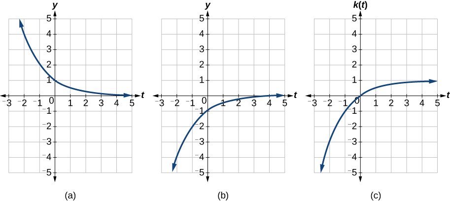
This equation combines three transformations into one equation.

• A horizontal reflection: [latex]f\left(-t\right)={2}^{-t}[/latex]
• A vertical reflection: [latex]\text{}-f\left(-t\right)=-{2}^{-t}[/latex]
• A vertical shift: [latex]\text{}-f\left(-t\right)+1=-{2}^{-t}+1[/latex]

We can sketch a graph by applying these transformations one at a time to the original function. Let us follow two points through each of the three transformations. We will choose the points (0, 1) and (1, 2).

1. First, we apply a horizontal reflection: (0, 1) (–1, 2).
2. Then, we apply a vertical reflection: (0, −1) (-1, –2).
3. Finally, we apply a vertical shift: (0, 0) (-1, -1).

This means that the original points, (0,1) and (1,2) become (0,0) and (-1,-1) after we apply the transformations.

In Figure 3-27, the first graph results from a horizontal reflection. The second results from a vertical reflection. The third results from a vertical shift up 1 unit.

Example 4: Graphing Functions

Notice: [latex]\text{}g\left(x\right)=f\left(-x\right)\text{}[/latex] looks the same as [latex]\text{}f\left(x\right)[/latex].

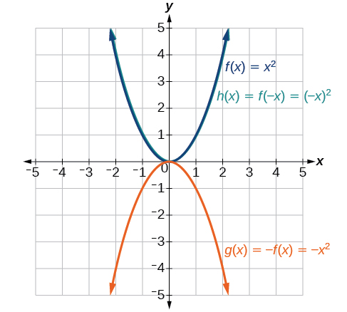
Example 1: Determining whether a Function Is Even, Odd, or Neither

1. Without looking at a graph, we can determine whether the function is even or odd by finding formulas for the reflections and determining if they return us to the original function. Let’s begin with the rule for even functions.

[latex]f\left(-x\right)={\left(-x\right)}^{3}+2\left(-x\right)=-{x}^{3}-2x[/latex]

This does not return us to the original function, so this function is not even. We can now test the rule for odd functions.

[latex]-f\left(-x\right)=-\left(-{x}^{3}-2x\right)={x}^{3}+2x[/latex]

Because[latex]\text{}-f\left(-x\right)=f\left(x\right),\text{}[/latex]this is an odd function.

2. even

Example 1: Graphing a Vertical Stretch

Because the population is always twice as large, the new population’s output values are always twice the original function’s output values. Graphically, this is shown in Figure 3-28.

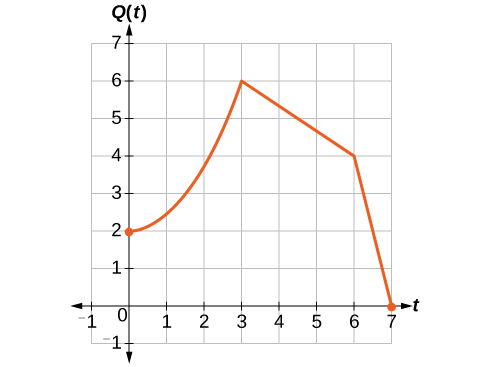
If we choose four reference points, (0, 1), (3, 3), (6, 2) and (7, 0) we will multiply all of the outputs by 2.

The following shows where the new points for the new graph will be located.

[latex]\begin{array}{l}\left(0,\text{ }1\right)\to \left(0,\text{ }2\right)\hfill \\ \left(3,\text{ }3\right)\to \left(3,\text{ }6\right)\hfill \\ \left(6,\text{ }2\right)\to \left(6,\text{ }4\right)\hfill \\ \left(7,\text{ }0\right)\to \left(7,\text{ }0\right)\hfill \end{array}[/latex]

Symbolically, the relationship is written as

[latex]Q\left(t\right)=2P\left(t\right)[/latex]

This means that for any input [latex]\text{}t\text{}[/latex], the value of the function [latex]\text{}Q\text{}[/latex] is twice the value of the function [latex]\text{}P\text{}[/latex]. Notice that the effect on the graph is a vertical stretching of the graph, where every point doubles its distance from the horizontal axis. The input values, [latex]\text{}t,\text{}[/latex] stay the same while the output values are twice as large as before.

Example 2: Finding a Vertical Compression of a Tabular Function

1. The formula [latex]\text{}g\left(x\right)=\frac{1}{2}f\left(x\right)\text{}[/latex] tells us that the output values of [latex]\text{}g\text{}[/latex] are half of the output values of [latex]\text{}f\text{}[/latex] with the same inputs. For example, we know that [latex]\text{}f\left(4\right)=3\text{}[/latex]. Then

[latex]g\left(4\right)=\frac{1}{2}f\left(4\right)=\frac{1}{2}\left(3\right)=\frac{3}{2}[/latex]

We do the same for the other values to produce Table 12.

Table 12

[latex]x[/latex]	[latex]2[/latex]	[latex]4[/latex]	[latex]6[/latex]	[latex]8[/latex]
[latex]g\left(x\right)[/latex]	[latex]\frac{1}{2}[/latex]	[latex]\frac{3}{2}[/latex]	[latex]\frac{7}{2}[/latex]	[latex]\frac{11}{2}[/latex]

2.

[latex]x[/latex]	2	4	6	8
[latex]g\left(x\right)[/latex]	9	12	15	0

Example 3: Recognizing a Vertical Stretch

When trying to determine a vertical stretch or shift, it is helpful to look for a point on the graph that is relatively clear. In this graph, it appears that [latex]\text{}g\left(2\right)=2\text{}[/latex]. With the basic cubic function at the same input, [latex]\text{}f\left(2\right)={2}^{3}=8\text{}[/latex]. Based on that, it appears that the outputs of [latex]\text{}g\text{}[/latex] are [latex]\text{}\frac{1}{4}\text{}[/latex] the outputs of the function [latex]\text{}f\text{}[/latex] because [latex]\text{}g\left(2\right)=\frac{1}{4}f\left(2\right)\text{}[/latex]. From this we can fairly safely conclude that [latex]\text{}g\left(x\right)=\frac{1}{4}f\left(x\right)[/latex].

We can write a formula for [latex]\text{}g\text{}[/latex] by using the definition of the function [latex]\text{}f[/latex].

[latex]g\left(x\right)=\frac{1}{4}f\left(x\right)=\frac{1}{4}{x}^{3}[/latex]

Example 4: Vertical Stretch

[latex]g\left(x\right)=3x-2[/latex]

Example 5: Graphing a Horizontal Compression

Symbolically, we could write

[latex]\begin{array}{l}R\left(1\right)=P\left(2\right),\hfill \\ R\left(2\right)=P\left(4\right),\text{ and in general,}\hfill \\ \text{}R\left(t\right)=P\left(2t\right).\hfill \end{array}[/latex]

See Figure 3-29 for a graphical comparison of the original population and the compressed population.

Example 6: Finding a Horizontal Stretch for a Tabular Function

The formula [latex]\text{}g\left(x\right)=f\left(\frac{1}{2}x\right)\text{}[/latex] tells us that the output values for [latex]\text{}g\text{}[/latex] are the same as the output values for the function [latex]\text{}f\text{}[/latex] at an input half the size. Notice that we do not have enough information to determine [latex]\text{}g\left(2\right)\text{}[/latex] because [latex]\text{}g\left(2\right)=f\left(\frac{1}{2}\cdot 2\right)=f\left(1\right)\text{}[/latex], and we do not have a value for [latex]\text{}f\left(1\right)\text{}[/latex] in our table. Our input values to [latex]\text{}g\text{}[/latex] will need to be twice as large to get inputs for [latex]\text{}f\text{}[/latex] that we can evaluate. For example, we can determine [latex]\text{}g\left(4\right)\text{}[/latex].

[latex]g\left(4\right)=f\left(\frac{1}{2}\cdot 4\right)=f\left(2\right)=1[/latex]

We do the same for the other values to produce Table 13.

Table 13

[latex]x[/latex]	4	8	12	16
[latex]g\left(x\right)[/latex]	1	3	7	11

Figure 3-30 shows the graphs of both of these sets of points.

Example 7: Recognizing a Horizontal Compression on a Graph

The graph of [latex]\text{}g\left(x\right)\text{}[/latex] looks like the graph of [latex]\text{}f\left(x\right)\text{}[/latex] horizontally compressed. Because [latex]\text{}f\left(x\right)\text{}[/latex] ends at [latex]\text{}\left(6,4\right)\text{}[/latex] and [latex]\text{}g\left(x\right)\text{}[/latex] ends at [latex]\text{}\left(2,4\right)\text{}[/latex], we can see that the [latex]\text{}x\text{-}[/latex]values have been compressed by [latex]\text{}\frac{1}{3}\text{}[/latex], because [latex]\text{}6\left(\frac{1}{3}\right)=2\text{}[/latex]. We might also notice that [latex]\text{}g\left(2\right)=f\left(6\right)\text{}[/latex] and [latex]\text{}g\left(1\right)=f\left(3\right)\text{}[/latex]. Either way, we can describe this relationship as [latex]\text{}g\left(x\right)=f\left(3x\right)\text{}[/latex]. This is a horizontal compression by [latex]\text{}\frac{1}{3}[/latex].

Example 8: Horizontal Stretch

[latex]g\left(x\right)=f\left(\frac{1}{3}x\right)\text{}[/latex] so using the square root function we get [latex]\text{}g\left(x\right)=\sqrt{\frac{1}{3}x}[/latex]

Example 9: Finding a Triple Transformation of a Tabular Function

There are three steps to this transformation, and we will work from the inside out. Starting with the horizontal transformations, [latex]\text{}f\left(3x\right)\text{}[/latex] is a horizontal compression by [latex]\text{}\frac{1}{3}\text{}[/latex], which means we multiply each [latex]\text{}x\text{-}[/latex]value by [latex]\text{}\frac{1}{3}[/latex]. See Table 14.

Table 14

[latex]x[/latex]	2	4	6	8
[latex]f\left(3x\right)[/latex]	10	14	15	17

Looking now to the vertical transformations, we start with the vertical stretch, which will multiply the output values by 2. We apply this to the previous transformation. See Table 15.

Table 15

[latex]x[/latex]	2	4	6	8
[latex]2f\left(3x\right)[/latex]	20	28	30	34

Finally, we can apply the vertical shift, which will add 1 to all the output values. See Table 16.

Table 16

[latex]x[/latex]	2	4	6	8
[latex]g\left(x\right)=2f\left(3x\right)+1[/latex]	21	29	31	35

Example 10: Finding a Triple Transformation of a Graph

To simplify, let’s start by factoring out the inside of the function.

[latex]f\left(\frac{1}{2}x+1\right)-3=f\left(\frac{1}{2}\left(x+2\right)\right)-3[/latex]

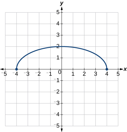
By factoring the inside, we can first horizontally stretch by 2, as indicated by the [latex]\text{}\frac{1}{2}\text{}[/latex] on the inside of the function. Remember that twice the size of 0 is still 0, so the point (0,2) remains at (0,2) while the point (2,0) will stretch to (4,0). See Figure 3-31.

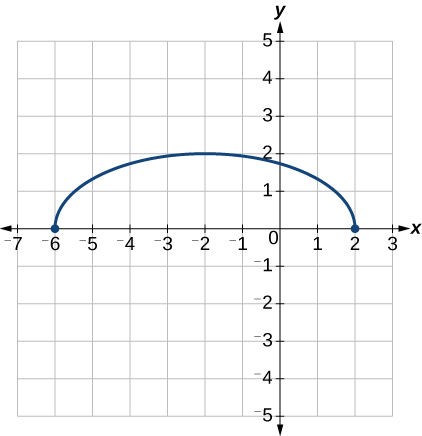
Next, we horizontally shift left by 2 units, as indicated by [latex]\text{}x+2\text{}[/latex]. See Figure 3-32.

Last, we vertically shift down by 3 to complete our sketch, as indicated by the [latex]\text{}-3\text{}[/latex] on the outside of the function. See Figure 3-33.